This blog post introduces the notion of “isometric invariant states” in Algebraic Quantum Field Theory (AQFT) in Minkowski spacetime (a theory defined in Unpacking the Haag Kastler Axioms) and also does the same for AQFT in Lorentzian spacetime (a theory defined in Haag Kastler Axioms in Curved Spacetime). Such “isometric invariant states” capture the physics of quantum systems that are invariant under isometries of spacetime.

Review of Algebraic Quantum Field Theory

Instead of diving headlong into a definition of “isometric invariant states”, we will begin with a review of AQFT in Minkowski spacetime and AQFT in Lorentzian spacetime.

The reviews of AQFT in Minkowski and Lorentzian spacetime will not provide all details of the blog posts Unpacking the Haag Kastler Axioms and Haag Kastler Axioms in Curved Spacetime where these theories were introduced. The AQFT reviews serve only as a refresher, making sure readers are clear on the various definitions and axioms used.

Algebraic Quantum Field Theory in Minkowski Spacetime

Now, before introducing any axioms that codify AQFT in Minkowski Spacetime, we must define Minkowski spacetime itself, the arena upon which everything unfolds.

Definition (Chronological Future and Past) Consider a point \(p\) in a smooth manifold with a Minkowski metric and associated time orientation. The chronological future of \(p\) is the set \(I^+(p)\) of points reachable from \(p\) via a future-directed, time-like curve. Similarly, the chronological past of \(p\) is the set \(I^-(p)\) of all points that reach \(p\) via a future-directed, time-like curve.

Definition (Minkowski Spacetime) Minkowski spacetime is the standard, smooth manifold \(\mathbb{R}^4\) equipped with the standard time orientation \((1,0,0,0)\), associated Minkowski metric, and associated Alexandrov topology. (Note the Alexandrov topology is the topology in which sets of the form \(I^+(p) \cap I^-(q)\) form the basis.)

That done we can introduce the first axiom of AQFT in Minkowski spacetime:

Axiom 1 (Local Algebras) For any basis element \(\mathbf{B}\) of the Alexandrov topology on Minkowski spacetime, i.e. any set of the form \(I^+(p) \cap I^-(q)\), there is a corresponding abstract C*-algebra \(\mathfrak{U}(\mathbf{B})\)

\[\mathbf{B} \longmapsto \mathfrak{U}(\mathbf{B}),\]

and when \(\mathbf{B}\) is the empty set, we have the distinguished correspondence

\[\emptyset \longmapsto \mathbb{C} \mathbf{1},\]

where \(\mathbf{1}\) is the multiplicative identity in the abstract C*-algebra \(\mathbb{C} \mathbf{1}\).

The second axiom takes the following form:

Axiom 2 (Isotony) Let \(\mathbf{B}_1\) and \(\mathbf{B}_2\) be any two basis elements of the Alexandrov topology on Minkowski spacetime, i.e. any two sets of the form \(I^+(p_1) \cap I^-(q_1)\) and \(I^+(p_2) \cap I^-(q_2)\).

If \(\mathbf{B}_1 \subset \mathbf{B}_2\) then \(\mathfrak{U}(\mathbf{B}_1) \subset \mathfrak{U}(\mathbf{B}_2)\), where inclusion is implemented by

\[i : \mathfrak{U}(\mathbf{B}_1) \hookrightarrow \mathfrak{U}(\mathbf{B}_2),\]

a unital *-monomorphism.

Before stating the next axiom, we need to introduce some terminology that appears therein.

Definition (Quasilocal Algebra) Consider the set-theoretic union of all \(\mathfrak{U}(\mathbf{B})\). As proven in the blog post (Unpacking the Haag Kastler Axioms), this set-theoretic union is a normed *-algebra. Also, as proven in the blog post (Unpacking the Haag Kastler Axioms), its completion yields a C*-algebra, denoted as \(\mathfrak{U}\). This C*-algebra \(\mathfrak{U}\) is called the quasilocal algebra.

Definition (Causal Future and Past) Consider a point \(p\) in a Minkowski spacetime. The causal future of \(p\) is the set \(J^+(p)\) of points reachable from \(p\) via a future-directed, time-like or light-like curve. Similarly, the causal past of \(p\) is the set \(J^-(p)\) of all points that reach \(p\) via a future-directed, time-like or light-like curve.

Definition (Spacelike Related) Consider two points \(p_1\) and \(p_2\) in a Minkowski spacetime. The points are said to be spacelike related if \(p_2 \notin J^+(p_1) \cup J^-(p_1)\) or equivalently \(p_1 \notin J^+(p_2) \cup J^-(p_2)\).

Definition (Completely Spacelike) Consider two sets \(\mathbf{O}_1\) and \(\mathbf{O}_2\) in a Minkowski spacetime. \(\mathbf{O}_1\) and \(\mathbf{O}_2\) are said to be completely spacelike if every \(p_1\) in \(\mathbf{O}_1\) is spacelike related to every \(p_2\) in \(\mathbf{O}_2\) or equivalently if every \(p_2\) in \(\mathbf{O}_2\) is spacelike related to every \(p_1\) in \(\mathbf{O}_1\).

With all of these definitions in hand, we can now state the next axiom:

Axiom 3 (Local Commutativity) Let \(\mathbf{B}_1\) and \(\mathbf{B}_2\) be any two basis elements of the Alexandrov topology on Minkowski spacetime, i.e. any two sets of the form \(I^+(p_1) \cap I^-(q_1)\) and \(I^+(p_2) \cap I^-(q_2)\).

If \(\mathbf{B_1}\) and \(\mathbf{B_2}\) are completely spacelike, then \(\mathfrak{U}(\mathbf{B_1})\) and \(\mathfrak{U}(\mathbf{B_2})\) commute in the quasilocal algebra \(\mathfrak{U}\), i.e. for any \(a_1\) in \(\mathfrak{U}(\mathbf{B_1})\) and \(a_2\) in \(\mathfrak{U}(\mathbf{B_2})\) it follows that

\[i(a_1) i(a_2) - i(a_2) i(a_1) = 0\]

in the quasilocal algebra \(\mathfrak{U}\).

The definitions required in the next axiom make use of terminology introduced in the previous blog post GNS Construction Theorem. It’s strongly recommended that the reader be familiar with the GNS Construction Theorem or read GNS Construction Theorem before proceeding.

That said, to state the next axiom we make use of the following definition:

Definition (Quasilocal Observable) The image \(\pi_\omega(a)\) of a self-adjoint member \(a\) of the quasilocal algebra \(\mathfrak{U}\) under a GNS *-homomorphism \(\pi_\omega\) of state \(\omega\) is self-adjoint and thus corresponds to an “observable”. Any “observable” corresponding to such a self-adjoint \(\pi_\omega(a)\) is called a quasilocal observable.

Using this definition we can then state the next axiom

Axiom 4 (Quasilocal Algebra) All “observables” are quasilocal observables.

Finally we can state the last axiom

Axiom 5 (Lorentz Covariance) Let \(\mathbf{B}\) be any basis element of the Alexandrov topology on Minkowski spacetime, i.e. any set of the form \(I^+(p) \cap I^-(q)\).

A member \(L\) of the inhomogeneous Lorentz group connected to the identity acts on \(\mathfrak{U}(\mathbf{B})\) as follows

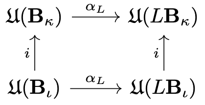
\[\begin{align} \alpha_L : \mathfrak{U}(\mathbf{B}) &\longrightarrow \mathfrak{U}(L\mathbf{B}) \\ a &\longmapsto \alpha_L(a) \end{align}\]

where \(L\mathbf{B}\) is the image of the region \(\mathbf{B}\) under the transformation \(L\) and \(\alpha_L\) is a unital *-isomorphism generated by \(L\). The map \(\alpha_L\) is such that (1) for the identity element \(\mathbf{1}\) of the Lorentz group it satisfies

\[\alpha_{\mathbf{1}}(a) = a,\]

(2) for all appropriate \(a\), \(L\), and \(L'\) it satisfies

\[\alpha_{L' \cdot L}(a) = \alpha_{L'}(\alpha_{L}(a)),\]

and (3) for basis elements \(\mathbf{B}_\iota \subset \mathbf{B}_\kappa\) and the unital *-monomorphism \(i\) of Axiom 2 (Isotony) \(\alpha_L\) commutes with \(i\). In other words the following diagram

commutes.

Algebraic Quantum Field Theory in Lorentzian Spacetime

The lightning review of AQFT in Minkowski spacetime complete, we now move onto a review of AQFT in Lorentzian spacetime.

As in the Minkowski case, before introducing any axioms that codify AQFT in Lorentzian spacetime, we need to specify exactly what Lorentzian spacetime is:

Definition (Chronological Future and Past) Consider a point \(p\) in a smooth manifold with a Lorentzian metric and associated time orientation. The chronological future of \(p\) is the set \(I^+(p)\) of points reachable from \(p\) via a future-directed, time-like curve. Similarly, the chronological past of \(p\) is the set \(I^-(p)\) of all points that reach \(p\) via a future-directed, time-like curve.

Definition (Lorentzian Spacetime) A Lorentzian spacetime is a smooth, connected, four dimensional manifold equipped with a smooth, nowhere-vanishing global vector field \(t^a\) and associated Lorentzian metric. In addition it is equipped with an associated Hausdorff Alexandrov topology.

That clarified, we can present the first axiom:

Axiom 1 (Local Algebras) For any basis element \(\mathbf{B}\) of the Alexandrov topology on a Lorentzian spacetime, i.e. any set of the form \(I^+(p) \cap I^-(q)\), there is a corresponding abstract C*-algebra \(\mathfrak{U}(\mathbf{B})\)

\[\mathbf{B} \longmapsto \mathfrak{U}(\mathbf{B}),\]

and when \(\mathbf{B}\) is the empty set, we have the distinguished correspondence

\[\emptyset \longmapsto \mathbb{C} \mathbf{1},\]

where \(\mathbf{1}\) is the multiplicative identity in the abstract C*-algebra \(\mathbb{C} \mathbf{1}\).

The second axiom can be immediately stated:

Axiom 2 (Isotony) Let \(\mathbf{B}_1\) and \(\mathbf{B}_2\) be any two basis elements of the Alexandrov topology on a Lorentzian spacetime, i.e. any two sets of the form \(I^+(p_1) \cap I^-(q_1)\) and \(I^+(p_2) \cap I^-(q_2)\).

If \(\mathbf{B}_1 \subset \mathbf{B}_2\) then \(\mathfrak{U}(\mathbf{B}_1) \subset \mathfrak{U}(\mathbf{B}_2)\), where inclusion is implemented by

\[i : \mathfrak{U}(\mathbf{B}_1) \hookrightarrow \mathfrak{U}(\mathbf{B}_2),\]

a unital *-monomorphism.

The next axiom makes use of the following definitions:

Definition (Causal Future and Past) Consider a point \(p\) in a Lorentzian spacetime. The causal future of \(p\) is the set \(J^+(p)\) of points reachable from \(p\) via a future-directed, time-like or light-like curve. Similarly, the causal past of \(p\) is the set \(J^-(p)\) of all points that reach \(p\) via a future-directed, time-like or light-like curve.

Definition (Spacelike Related) Consider two points \(p_1\) and \(p_2\) in a Lorentzian spacetime. The points are said to be spacelike related if \(p_2 \notin J^+(p_1) \cup J^-(p_1)\) or equivalently \(p_1 \notin J^+(p_2) \cup J^-(p_2)\).

Definition (Completely Spacelike) Consider two sets \(\mathbf{O}_1\) and \(\mathbf{O}_2\) in a Lorentzian spacetime. \(\mathbf{O}_1\) and \(\mathbf{O}_2\) are said to be completely spacelike if every \(p_1\) in \(\mathbf{O}_1\) is spacelike related to every \(p_2\) in \(\mathbf{O}_2\) or equivalently if every \(p_2\) in \(\mathbf{O}_2\) is spacelike related to every \(p_1\) in \(\mathbf{O}_1\).

and can be stated as follows:

Axiom 3 (Local Commutativity) Let \(\mathbf{B}_1\) and \(\mathbf{B}_2\) be any two basis elements of the Alexandrov topology on a Lorentzian spacetime, i.e. any two sets of the form \(I^+(p_1) \cap I^-(q_1)\) and \(I^+(p_2) \cap I^-(q_2)\).

If \(\mathbf{B_1}\) and \(\mathbf{B_2}\) are completely spacelike, for any basis element \(\mathbf{B}\) such that \(\mathbf{B_1}, \mathbf{B_2} \subseteq \mathbf{B}\) the algebras \(\mathfrak{U}(\mathbf{B_1})\) and \(\mathfrak{U}(\mathbf{B_2})\) commute in the C*-algebra \(\mathfrak{U}(\mathbf{B})\), i.e. for any \(a_1\) in \(\mathfrak{U}(\mathbf{B_1})\) and \(a_2\) in \(\mathfrak{U}(\mathbf{B_2})\) we have

\[i(a_1) i(a_2) - i(a_2) i(a_1) = 0\]

in the C*-algebra \(\mathfrak{U}(\mathbf{B})\).

If no such \(\mathbf{B}\) exists, then it simply doesn’t make sense to consider if \(\mathfrak{U}(\mathbf{B_1})\) and \(\mathfrak{U}(\mathbf{B_2})\) commute as they are not in the same algebra.

Again, the definitions required for the next axiom use terminology introduced in the previous blog post GNS Construction Theorem. It’s strongly recommended that the reader be familiar with the GNS Construction Theorem or read GNS Construction Theorem before proceeding.

That being said, the next axiom has need of the following definition:

Definition (Local Observable) For Lorentzian spacetime \(M\) the image \(\pi_\omega(a)\) of a self-adjoint member \(a\) of the local algebra \(\mathfrak{U}(\mathbf{B})\) under the GNS *-homomorphism \(\pi_\omega\) of a state \(\omega\) on \(\mathfrak{U}(\mathbf{B})\) is self-adjoint and thus corresponds to an “observable”. Any “observable” corresponding to such a self-adjoint \(\pi_\omega(a)\) is called a local observable.

and can be stated as follows:

Axiom 4 (Local Algebra) All “observables” are local observables.

The final axiom states:

Axiom 5 (Isometric Covariance) Let \(\mathbf{B}\) be any basis element of the Alexandrov topology on a Lorentzian spacetime \(M\), i.e. any set of the form \(I^+(p) \cap I^-(q)\).

A member \(\varphi\) of the group of isometries of \(M\) connected to the identity acts on \(\mathfrak{U}(\mathbf{B})\) as follows

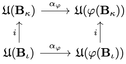
\[\begin{align} \alpha_\varphi : \mathfrak{U}(\mathbf{B}) &\longrightarrow \mathfrak{U}(\varphi(\mathbf{B})) \\ a &\longmapsto \alpha_\varphi(a) \end{align}\]

where \(\varphi(\mathbf{B})\) is the image of the basis element \(\mathbf{B}\) under the isometry \(\varphi\) and \(\alpha_\varphi\) is a unital *-isomorphism generated by \(\varphi\). The map \(\alpha_\varphi\) is such that (1) for the identity isometry \(\mathbf{1}\) it satisfies

\[\alpha_{\mathbf{1}}(a) = a,\]

(2) for all appropriate \(a\), \(\varphi\), and \(\varphi'\) it satisfies

\[\alpha_{\varphi' \cdot \varphi}(a) = \alpha_{\varphi'}(\alpha_{\varphi}(a)),\]

and (3) for basis elements \(\mathbf{B}_\iota \subset \mathbf{B}_\kappa\) and the unital *-monomorphism \(i\) of Axiom 2 (Isotony) \(\alpha_\varphi\) commutes with \(i\). In other words the following diagram

commutes.

Introduction to States

In this section we will examine various types of states with the goal of eventually introducing “global isometric invariant states” and “local isometric invariant states”, the “local” case being of most physical relevance.

Abstract C*-Algebra States

Before introducing the various states associated with AQFT, we will take a moment to remind the reader of the definition of an abstract C*-algebra state that was introduced in the blog post GNS Construction Theorem

Definition (State) Let \(\mathcal{C}\) be an abstract C*-algebra. A state is an element \(\omega\) of the dual space \(\mathcal{C}^*\) that is

• Positive - for any \(a \in \mathcal{C}\) we have \(0 \le \omega(a^*a)\) and
• Normalized - the operator norm satisfies \(\| \omega \|=1\).

Furthermore, a state \(\omega\) is said to be faithful if for any non-zero \(a\) in \(\mathcal{C}\), it follows that \(0 < \omega(a^*a)\).

This definition is critical; all subsequent notions of state associated with AQFT are built upon it.

States of Algebraic Quantum Field Theory in Minkowski Spacetime

In this section we detail how some notions of state in AQFT in Minkowski spacetime follow “naturally” from the notion of state for an abstract C*-algebra.

“Local states” in AQFT on Minkowski spacetime are simply abstract C*-algebra states associated to a local algebra \(\mathfrak{U}(\mathbf{B})\), where \(\mathbf{B}\) is a basis element of the Alexandrov topology in Minkowski spacetime. Similarly, “global states” there are abstract C*-algebra states associated to the quasilocal algebra \(\mathfrak{U}\).

These are “simple” extensions of the notion of an abstract C*-algebra state. These extensions start to become interesting only when we examine how they behave under isometries.

Local States of Algebraic Quantum Field Theory in Minkowski Spacetime

Formally a “local state” of AQFT in Minkowski Spacetime is defined as follows:

Definition (Local State) Let \(\mathbf{B}\) be any basis element of the Alexandrov topology in Minkowski spacetime, i.e. any set of the form \(I^+(p) \cap I^-(q)\), and \(\mathfrak{U}(\mathbf{B})\) its associated abstract C*-algebra.

A local state is an element \(\omega\) of the dual space \(\mathfrak{U}(\mathbf{B})^*\) that is

• Positive - for any \(a \in \mathfrak{U}(\mathbf{B})\) we have \(0 \le \omega(a^*a)\) and
• Normalized - the operator norm satisfies \(\| \omega \|=1\).

Furthermore, a local state \(\omega\) is said to be faithful if for any non-zero \(a\) in \(\mathfrak{U}(\mathbf{B})\), it follows that \(0 < \omega(a^*a)\).

Thus a local state is “simply” an abstract C*-algebra state associated to a local algebra \(\mathfrak{U}(\mathbf{B})\).

Global States of Algebraic Quantum Field Theory in Minkowski Spacetime

Similarly, a “global state” of AQFT in Minkowski Spacetime is defined as follows:

Definition (Global State) Let \(\mathfrak{U}\) be the quasilocal algebra associated with Minkowski spacetime.

A global state is an element \(\omega\) of the dual space \(\mathfrak{U}^*\) that is

• Positive - for any \(a \in \mathfrak{U}\) we have \(0 \le \omega(a^*a)\) and
• Normalized - the operator norm satisfies \(\| \omega \|=1\).

Furthermore, a global state \(\omega\) is said to be faithful if for any non-zero \(a\) in \(\mathfrak{U}\), it follows that \(0 < \omega(a^*a)\).

So, a global state is just an abstract C*-algebra state associated to the quasilocal algebra \(\mathfrak{U}\).

States of Algebraic Quantum Field Theory in Lorentzian Spacetime

The states associated to AQFT in Lorentzian spacetime also follow “naturally” from the definition of an abstract C*-algebra state.

“Local states” are abstract C*-algebra states associated to a “local” algebra. And in contrast to Minkowski spacetime, there exists no notion of “global states” in Lorentzian spacetime as there exists no quasilocal algebra associated with a general Lorentzian spacetime.

Local States of Algebraic Quantum Field Theory in Lorentzian Spacetime

Formally a “local state” of AQFT in a Lorentzian spacetime is

Definition (Local State) Let \(\mathbf{B}\) be any basis element of the Alexandrov topology in a Lorentzian spacetime, i.e. any set of the form \(I^+(p) \cap I^-(q)\), and \(\mathfrak{U}(\mathbf{B})\) its associated abstract C*-algebra.

A local state is an element \(\omega\) of the dual space \(\mathfrak{U}(\mathbf{B})^*\) that is

• Positive - for any \(a \in \mathfrak{U}(\mathbf{B})\) we have \(0 \le \omega(a^*a)\) and
• Normalized - the operator norm satisfies \(\| \omega \|=1\).

Furthermore, a local state \(\omega\) is said to be faithful if for any non-zero \(a\) in \(\mathfrak{U}(\mathbf{B})\), it follows that \(0 < \omega(a^*a)\).

So a local state is just an abstract C*-algebra state associated to a local algebra \(\mathfrak{U}(\mathbf{B})\). Furthermore, as there exists no quasilocal algebra associated with a general Lorentzian spacetime, there is no such thing as a “global state” on a generic Lorentzian spacetime.

Introduction to Isometric Invariant States

Finally, we’ve reached the “core” of this blog post, the study of “isometric invariant” states. As one might guess, “isometric invariant” states are local or global states that are “invariant” under spacetime isometries.

These states are interesting for many reasons. For example, they provide a canonical example of how one can create a state “invariant” under a given classical symmetry. Critically, “isometric invariant” states, with some additional properties, can also serve as AQFT vacua. In addition, they provide a laboratory in which to examine aspects of spontaneous symmetry breaking: e.g. Are the classical spacetime isometries broken by a quantum state?

With this as motivation, let’s jump right in!

Global Isometric Invariant States in Minkowski Spacetime

We begin with global, “isometric invariant” states in Minkowski spacetime. They are, in some sense, the “simplest” “isometric invariant” states. However, a careful examination of such global, “isometric invariant” states in Minkowski spacetime clarifies essentially all subtleties that arise in other cases.

Isometries of the Quasilocal Algebra

“Morally”, as the metric doesn’t change under an isometry, an isometry \(L\) of Minkowski spacetime, in particular a member of the inhomogeneous Lorentz group connected to the identity, should generate an associated unital *-automorphism \(\alpha_L\) of the quasilocal algebra \(\mathfrak{U}\)

and a global, “isometric invariant” state should be a global state \(\omega\) that is invariant with respect to this unital *-automorphism

While “morally” this is indeed the case, the problem one immediately encounters is that Axiom 5 (Lorentz Covariance) states only

Axiom 5 (Lorentz Covariance) Let \(\mathbf{B}\) be any basis element of the Alexandrov topology on Minkowski spacetime, i.e. any set of the form \(I^+(p) \cap I^-(q)\).

A member \(L\) of the inhomogeneous Lorentz group connected to the identity acts on \(\mathfrak{U}(\mathbf{B})\) as follows

\[\begin{align} \alpha_L : \mathfrak{U}(\mathbf{B}) &\longrightarrow \mathfrak{U}(L\mathbf{B}) \\ a &\longmapsto \alpha_L(a) \end{align}\]

where \(L\mathbf{B}\) is the image of the region \(\mathbf{B}\) under the transformation \(L\) and \(\alpha_L\) is a unital *-isomorphism generated by \(L\). The map \(\alpha_L\) is such that (1) for the identity element \(\mathbf{1}\) of the Lorentz group it satisfies

\[\alpha_{\mathbf{1}}(a) = a,\]

(2) for all appropriate \(a\), \(L\), and \(L'\) it satisfies

\[\alpha_{L' \cdot L}(a) = \alpha_{L'}(\alpha_{L}(a)),\]

and (3) for basis elements \(\mathbf{B}_\iota \subset \mathbf{B}_\kappa\) and the unital *-monomorphism \(i\) of Axiom 2 (Isotony) \(\alpha_L\) commutes with \(i\). In other words the following diagram

commutes.

So, the unital *-automorphism

isn’t defined by this axiom. Our first task, then, is to define this unital *-automorphism.

This task begins by recounting the definition of the quasilocal algebra

Definition (Quasilocal Algebra) Consider the set-theoretic union of all \(\mathfrak{U}(\mathbf{B})\). As proven in the blog post (Unpacking the Haag Kastler Axioms), this set-theoretic union is a normed *-algebra. Also, as proven in the blog post (Unpacking the Haag Kastler Axioms), its completion yields a C*-algebra, denoted as \(\mathfrak{U}\). This C*-algebra \(\mathfrak{U}\) is called the quasilocal algebra.

This implies that the set-theoretic union of all \(\mathfrak{U}(\mathbf{B})\) is dense in \(\mathfrak{U}\). Hence, if we can define \(\alpha_L\) on this set-theoretic union, then we should be able to employ the Bounded Linear Transformation Theorem (Theorem A.36 Hall)

Theorem (Bounded Linear Transformation Theorem) Let \(V_1\) be a normed space and \(V_2\) a Banach space. Suppose \(W\) is a dense subspace of \(V_1\) and \(T: W \rightarrow V_2\) is a bounded linear map. Then there exists a unique bounded linear map \(\widetilde{T}: V_1 \rightarrow V_2\) such that \(\widetilde{T}|_W = T\). Furthermore, the norm of \(\widetilde{T}\) equals the norm of \(T\).

to extend \(\alpha_L\) to the entire quasilocal algebra, the desired result. It is to this argument we now turn.

The first step in this argument is to prove the following theorem

Theorem On Minkowski spacetime let \(L\) be any member of the inhomogeneous Lorentz group that is connected to the identity and let

\[\{ \mathbf{B}_\iota \}_{\iota \in \mathcal{I}}\]

be the set of all elements \(\mathbf{B}_\iota\) of the form \(I^+(p_\iota) \cap I^-(q_\iota)\) in Minkowski spacetime.

Then there exists a map

\[\alpha_L : \bigcup\limits_{\iota \in \mathcal{I}} \mathfrak{U}(\mathbf{B}_\iota) \longrightarrow \mathfrak{U}\]

from the set theoretic union over all \(\mathfrak{U}(\mathbf{B}_\iota)\) to the quasilocal algebra \(\mathfrak{U}\) such that: (1) The map \(\alpha_L\) is linear; (2) The map \(\alpha_L\) is bounded; and (3) The restriction of \(\alpha_L\) to any \(\mathfrak{U}(\mathbf{B}_\iota)\)

\[\left. \alpha_L\right|_{\mathfrak{U}(\mathbf{B}_\iota)} : \mathfrak{U}(\mathbf{B}_\iota) \longrightarrow \mathfrak{U}(L\mathbf{B}_\iota)\]

is the map that appears in Axiom 5 (Lorentz Covariance).

Proof First will prove that there exists a linear map \(\alpha_L\) of the desired form

where the union is over all sets \(\mathbf{B}_\iota\) of the form \(I^+(p_\iota) \cap I^-(q_\iota)\) in Minkowski spacetime.

Let us start by explicitly defining the domain of \(\alpha_L\), the set theoretic union over all \(\mathfrak{U}(\mathbf{B}_\iota)\).

Consider first the disjoint union over all \(\mathfrak{U}(\mathbf{B}_\iota)\)

As a result of Axiom 2 (Isotony), we can define an equivalence relation over this disjoint union, which we now proceed to do.

Consider two elements \(a_\iota\) and \(a_\kappa\) of this disjoint union. The definition of disjoint union implies that there exist two sets \(\mathbf{B}_\iota\) and \(\mathbf{B}_\kappa\) such that \(a_\iota \in \mathfrak{U}(\mathbf{B}_\iota)\) and \(a_\kappa \in \mathfrak{U}(\mathbf{B}_\kappa)\). The two elements \(a_\iota\) and \(a_\kappa\) are defined to be equivalent if \(\mathbf{B}_\iota \subset \mathbf{B}_\kappa\) and thus \(\mathfrak{U}(\mathbf{B}_\iota) \subset \mathfrak{U}(\mathbf{B}_\kappa)\) and in addition \(a_\iota\) and \(a_\kappa\) are related as follows \(i(a_\iota) = a_\kappa\) by the unital *-monomorphism \(i\) of Axiom 2 (Isotony).

The set theoretic union over all \(\mathfrak{U}(\mathbf{B}_\iota)\) is defined as the disjoint union mod this equivalence relation

This is the domain of \(\alpha_L\) and it is, by definition, a subset of the quasilocal algebra \(\mathfrak{U}\).

Next let us define how \(\alpha_L\) acts on this set theoretic union.

Consider an element \([a]\) in this set theoretic union. Let \(a\) be any representative of the equivalence class \([a]\). Thus there exists a \(\mathbf{B}\) such that \(a\) is an element in \(\mathfrak{U}(\mathbf{B})\). Axiom 5 (Lorentz Covariance) implies that there exists a unital *-isomorphism \(\alpha_L\)

that can act on \(a\). We then define the action of our desired \(\alpha_L\) on \([a]\) as follows

In other words

To prove this is well-defined we must prove that it is independent of which representative \(a\) of the equivalence class \([a]\) is used in this definition. Proving this is relatively easy.

Axiom 5 (Lorentz Covariance) states that the unital *-monomorphism \(i\) of Axiom 2 (Isotony) commutes with the unital *-isomorphism \(\alpha_L\). Hence, if we were to select any other representative \(i(a)\) of the equivalence class to define the action of \(\alpha_L\) on the set theoretic union we would have

giving the same result as before and proving that our definition of \(\alpha_L\) is well-defined.

As an aside, note that the range of our map

makes sense as the definition of the quasilocal algebra \(\mathfrak{U}\) states that the set theoretic union is a subset of \(\mathfrak{U}\) and \([\alpha_L(a)]\) is a member of the set theoretic union.

Now we need to prove \(\alpha_L\) is linear.

Consider two elements \([a]\) and \([b]\) in the set theoretic union as well as two elements \(\lambda\) and \(\mu\) of \(\mathbb{C}\). Let \(a\) be a representative of the equivalence class \([a]\) and \(b\) a representative of the equivalence class \([b]\). Thus there exists a \(\mathbf{B}_a\) such that \(a\) is an element in \(\mathfrak{U}(\mathbf{B}_a)\) and \(\mathbf{B}_b\) such that \(b\) is in \(\mathfrak{U}(\mathbf{B}_b)\).

As we are in Minkowski spacetime there exists a \(\mathbf{B}\) of the form \(I^+(p) \cap I^-(q)\) such that \(\mathbf{B}_a, \mathbf{B}_b \subseteq \mathbf{B}\). Via Axiom 5 (Lorentz Covariance) we also have the associated unital *-isomorphism

As this \(\alpha_L\) is a unital *-isomorphism, it is linear. Axiom 2 (Isotony) implies that \(\mathfrak{U}(\mathbf{B}_a), \mathfrak{U}(\mathbf{B}_b) \subset \mathfrak{U}(\mathbf{B})\). So all of this together implies

where the first equality employs the definition of \(\alpha_L\) acting on the set theoretic union in terms of \(\alpha_L\) acting on \(\mathfrak{U}(\mathbf{B})\), the second equality uses the linearity of \(\alpha_L\) acting on \(\mathfrak{U}(\mathbf{B})\), and the final line uses the definition of \(\alpha_L\) acting on the set theoretic union in terms of \(\alpha_L\) acting on \(\mathfrak{U}(\mathbf{B})\). This proves \(\alpha_L\) acting on the set theoretic union is linear, the desired result.

Note in the subsequent text we will rarely use the equivalence class \([a]\) notation for members of the set theoretic union. We will simply use \(a\). While it’s technically correct to use \([a]\), the exposition is “far cleaner” using \(a\), and, as we have seen, results are independent of the equivalence class representative selected. So nothing is lost in using \(a\).

Now let us prove that our map

is bounded.

We begin this part of the proof by proving the following lemma

Lemma (Spectral Equivalence) Let \(\mathfrak{U}_1\) and \(\mathfrak{U}_2\) be unital C*-algebras, \(\alpha: \mathfrak{U} \rightarrow \mathfrak{U}_2\) a unital *-monomorphism where \(\mathfrak{U} \subseteq \mathfrak{U}_1\), and \(a_1\) an arbitrary element of \(\mathfrak{U}\).

Then it follows that

\[\sigma(\alpha(a_1)) = \sigma(a_1).\]

In other words, the spectrum \(\sigma(\alpha(a_1))\) of \(\alpha(a_1)\) in \(\mathfrak{U}_2\) is equivalent to the spectrum \(\sigma(a_1)\) of \(a_1\) in \(\mathfrak{U}_1\).

Proof Consider \(\lambda \notin \sigma(a_1)\). The definition of spectrum then implies that \((a_1 - \lambda \mathbf{1}_{\mathfrak{U}_1})\) is invertible in \(\mathfrak{U}_1\). Let \((a_1 - \lambda \mathbf{1}_{\mathfrak{U}_1})^{-1}\) be that inverse. As \(\alpha\) is a unital *-monomorphism

Similarly, as \(\alpha\) is a unital *-monomorphism

Combining the previous two derivations

Thus, \((\alpha(a_1) - \lambda \mathbf{1}_{\mathfrak{U}_2})\) is invertible in \(\mathfrak{U}_2\), and thus \(\lambda \notin \sigma(\alpha(a_1))\). This then implies

Now as \(\alpha\) is a unital *-monomorphism, it follows that when \(\alpha\) is restricted to domain \(\mathfrak{U}\) and range \(\alpha(\mathfrak{U})\), it is invertible. Thus

is well-defined. Thus,

where \(\alpha(\mathfrak{U}) \subseteq \mathfrak{U}_2\), is a unital *-monomorphism. Hence, we can repeat the above argument using \(\alpha^{-1}\) with domain \(\alpha(\mathfrak{U})\) to conclude

So, we have proven that \(\sigma(\alpha(a_1)) \subseteq \sigma(a_1)\) and that \(\sigma(a_1) \subseteq \sigma(\alpha(a_1))\). Together these imply the desired result \(\sigma(\alpha(a_1)) = \sigma(a_1)\). \(\blacksquare\)

The next result we need to establish on the road to proving that \(\alpha_L\) is bounded is the following

Lemma Let \(\mathfrak{U}_1\) and \(\mathfrak{U}_2\) be unital C*-algebras, \(\alpha: \mathfrak{U} \rightarrow \mathfrak{U}_2\) a unital *-monomorphism where \(\mathfrak{U} \subseteq \mathfrak{U}_1\), and \(a_1\) an arbitrary self-adjoint element of \(\mathfrak{U}\).

Then it follows that

\[\|\alpha(a_1)\| = \|a_1\|\]

Proof Recall the following lemma (Lemma 8.1 Hall)

Lemma If \(a\) is a self-adjoint member of a unital C*-algebra, then its norm \(\|a\|\) is equivalent to its spectral radius \(r(a)\), i.e.

\[\|a\| = r(a).\]

Hence,

as a result of this lemma.

As \(\alpha\) is a unital *-monomorphism and \(a_1\) is self-adjoint

i.e. \(\alpha(a_1)\) is also self-adjoint. Hence, the previous lemma implies

Now the definition of spectral radius along with our Spectral Equivalence Theorem imply

Thus \(r(\alpha(a_1)) = r(a_1)\). This along with \(\|\alpha(a_1)\| = r(\alpha(a_1))\) and \(\|a_1\| = r(a_1)\) imply

the desired result. \(\blacksquare\)

As proven in the blog post (Unpacking the Haag Kastler Axioms) the quasilocal algebra \(\mathfrak{U}\) is a C*-algebra. Also, the definition of the quasilocal algebra \(\mathfrak{U}\) implies

Furthermore, Axiom 5 (Lorentz Covariance) and our construction of the map

imply that this map \(\alpha_L\) is a unital *-monomorphism.

One can see \(\alpha_L\) is a unital *-monomorphism by looking at its definition

As \(\alpha_L\) on the righthand side is a unital *-isomorphism we have

which implies \(\alpha_L([a])\) is unital. A similar argument, relying upon the the fact that \(\alpha_L\) on the righthand side of

is a unital *-isomorphism and the set theoretic union being a subset of \(\mathfrak{U}\), implies that the map \(\alpha_L([a])\) is a unital *-monomorphism.

Hence, we can apply the previous lemma to an arbitrary self-adjoint element of the set theoretic union. To that end consider an arbitrary element \(a\) in the set theoretic union

The element \(a\) need not be self-adjoint. However, \(a^*a\) is self-adjoint. Thus using C*-norm properties along with the fact that the “local” \(\alpha_L\) used to define \(\alpha_L\) are unital *-isomorphisms, we have

This implies

In other words, \(\alpha_L\) is an isometry.

Now, by definition

Using the results of the last paragraph this becomes

In other words \(\|\alpha_L\| = 1\) and thus \(\alpha_L\) is bounded, the second desired result.

The final desired result—i.e. the restriction of \(\alpha_L\) acting on the set theoretic union to any \(\mathfrak{U}(\mathbf{B}_\iota)\)

is the map that appears in Axiom 5 (Lorentz Covariance)—follows obviously from our construction of \(\alpha_L\). \(\blacksquare\)

So, as we have established that our \(\alpha_L\) is linear, bounded, and reduces to \(\alpha_L\) from Axiom 5 (Lorentz Covariance) in the appropriate limit, we now want to apply the Bounded Linear Transformation Theorem (Theorem A.36 Hall)

Theorem (Bounded Linear Transformation Theorem) Let \(V_1\) be a normed space and \(V_2\) a Banach space. Suppose \(W\) is a dense subspace of \(V_1\) and \(T: W \rightarrow V_2\) is a bounded linear map. Then there exists a unique bounded linear map \(\widetilde{T}: V_1 \rightarrow V_2\) such that \(\widetilde{T}|_W = T\). Furthermore, the norm of \(\widetilde{T}\) equals the norm of \(T\).

to uniquely extend

to

as a unital *-automorphism.

In applying this theorem \(\mathfrak{U}\), being a C*-algebra and thus normed space, takes on the role of \(V_1\). Similarly, \(\mathfrak{U}\), being a C*-algebra and thus Banach space, also takes on the role of \(V_2\). In addition \(\alpha_L\), being bounded and linear, takes on the role of \(T\). Finally,

takes on the role of \(W\) as it is dense in \(\mathfrak{U}\).

So with this we can then apply the Bounded Linear Transformation Theorem and uniquely extend

to

Now we must prove that this extension is indeed a unital *-automorphism. In other words we must prove the following theorem

Theorem The extension

\[\alpha_L : \mathfrak{U} \longrightarrow \mathfrak{U}\]

of the unital *-monomorphism

\[\alpha_L : \bigcup\limits_{\iota \in \mathcal{I}} \mathfrak{U}(\mathbf{B}_\iota) \longrightarrow \mathfrak{U}\]

to the domain \(\mathfrak{U}\) by the Bounded Linear Transformation Theorem is a unital *-automorphism.

Proof Proving the extension \(\alpha_L\) is a unital *-automorphism involves several steps: (1) proving it is a *-homomorphism, (2) proving it is unital, (3) proving it is injective, and (4) proving it is surjective. Together these results will prove that the extension is a unital *-automorphism.

Let us first (1) prove the extension \(\alpha_L\) is a *-homomorphism.

Proving the extension \(\alpha_L\) is a *-homomorphism involves (1a) proving \(\alpha_L(ab) = \alpha_L(a)\alpha_L(b)\) and (1b) proving \(\alpha_L(a^*)=\alpha_L(a)^*\) for arbitrary \(a\) and \(b\) in the quasilocal algebra \(\mathfrak{U}\).

Let us first prove that \(\alpha_L(ab) = \alpha_L(a)\alpha_L(b)\).

Let \(a\) and \(b\) be arbitrary elements of \(\mathfrak{U}\). As the set theoretic union is dense in \(\mathfrak{U}\) there exists a sequence \((a_i)_{i=1}^\infty\) in the the set theoretic union that converges to \(a\) and a sequence \((b_i)_{i=1}^\infty\) in the the set theoretic union that converges to \(b\).

As a result of the fact that \(\mathfrak{U}\) is a C*-algebra, for arbitrary \(c\) and \(d\) in \(\mathfrak{U}\) one has

This implies that multiplication in \(\mathfrak{U}\) is jointly continuous. Hence,

Now the Bounded Linear Transformation Theorem implies that the extension \(\alpha_L\) is continuous. Hence,

As \(a_i\) and \(b_i\) are in the set theoretic union, the extension and original \(\alpha_L\) agree on the set theoretic union, and the original \(\alpha_L\) is a unital *-monomorphism, we can continue the derivation as follows

However, joint continuity implies

Putting everything together we have proven

In other words, the extension \(\alpha_L\) is a homomorphism.

Let us next prove that the extension satisfies \(\alpha_L(a^*)=\alpha_L(a)^*\).

This proof is similar. Let \(a\) be an arbitrary element of \(\mathfrak{U}\). As the set theoretic union is dense in \(\mathfrak{U}\) there exists a sequence \((a_i)_{i=1}^\infty\) in the the set theoretic union that converges to \(a\).

As the extension \(\alpha_L\) is continuous and the unextended \(\alpha_L\) is a unital *-monomorphism we have

proving that the extension \(\alpha_L\) is not only a homomorphism but is a *-homomorphism.

Next let us (2) prove the extension \(\alpha_L\) is unital.

This proof is easier than the previous step.

The identity \(\mathbf{1}\) is in the set theoretic union, the extension \(\alpha_L\) and unextended \(\alpha_L\) agree on the set theoretic union, and the unextended \(\alpha_L\) is a unital *-monomorphism. This immediately results in

where the first equality follows from the fact that the extended and unextended \(\alpha_L\) agree on the set theoretic union and the second equality follows from the fact that the unextended \(\alpha_L\) is a unital *-monomorphism. This proves the extension \(\alpha_L\) is unital.

Next let us (3) prove the extension \(\alpha_L\) is injective.

Proving the extension \(\alpha_L\) is injective consists in (3a) proving it is an isometry \(\|\alpha_L(a)\| = \|a\|\) and (3b) proving the fact it is an isometry implies it is injective.

Let us first prove that \(\|\alpha_L(a)\| = \|a\|\).

As we previously proved that the unextended \(\alpha_L\) is an isometry, the goal of the current proof is to extend this result to all of \(\mathfrak{U}\).

Let \(a\) be an arbitrary element of the quasilocal algebra \(\mathfrak{U}\). As the set theoretic union is dense in \(\mathfrak{U}\), there exists a sequence \((a_i)_{i=1}^\infty\) in the the set theoretic union that converges to \(a\). The continuity of the extended \(\alpha_L\) then implies

Now as the extended and unextended \(\alpha_L\) agree on the set theoretic union and the unextended \(\alpha_L\) is an isometry, we can continue the derivation as follows

Putting this all together we have proven \(\|\alpha_L(a)\| = \|a\|\) which is none other than the statement that the extended \(\alpha_L\) is an isometry.

Next we will prove that the extended \(\alpha_L\) is injective.

To prove that the extended \(\alpha_L\) is injective, we must prove that its kernel is trivial. So, to that end let \(a\) be an element of its kernel. By definition \(\alpha_L(a) = 0\). Hence, \(\|\alpha_L(a)\| = 0\). However, as \(\alpha_L\) is an isometry this implies

This implies \(\|a\|=0\) and thus \(a=0\). Hence, it implies that the kernel of the extended \(\alpha_L\) is trivial, i.e. consists only of the zero element. This in turn implies that the extended \(\alpha_L\) is injective, the desired result.

Next let us (4) prove that the extended \(\alpha_L\) is surjective.

First note that as the extended \(\alpha_L\) is an isometry, it maps Cauchy sequences to Cauchy sequences. As its domain \(\mathfrak{U}\) is a C*-algebra, \(\mathfrak{U}\) is complete. Thus, the image \(\alpha_L(\mathfrak{U})\) of the complete space \(\mathfrak{U}\) is closed in \(\mathfrak{U}\).

The definition of the unextended \(\alpha_L\) in terms of the unital *-isomorphisms of Axiom 5 (Lorentz Covariance) implies

As the image of this unextended \(\alpha_L\) is in \(\alpha_L(\mathfrak{U})\) we can extend this equation as follows

As \(L\) is a group element and thus invertible and the union is over all elements \(\mathbf{B}_\iota\), the original set theoretic union is a subset of the left most term,

Thus we can conclude

Now as the set theoretic union is dense in \(\mathfrak{U}\), taking the closure of this equation gives

However, we just proved that \(\alpha_L(\mathfrak{U})\) is closed. Thus we can conclude

But, we know also that \(\alpha_L(\mathfrak{U}) \subseteq \mathfrak{U}\) and thus

which implies \(\alpha_L(\mathfrak{U}) = \mathfrak{U}\). In other words \(\alpha_L\) is surjective, the desired result.

Now we have proven that the extended \(\alpha_L\) is a unital *-homomorphism that is an injective and surjective map of \(\mathfrak{U}\) to itself. Thus by definition it is a unital *-automorphism, the desired result. \(\blacksquare\)

Definition of Global Isometric Invariant States

As we have established the definition of the unital *-automorphism

corresponding to any member \(L\) of the inhomogeneous Lorentz group that is connected to the identity, we are now in the position to define a global “isometric invariant” state

Definition (Global Isometric Invariant State) Let \(\mathfrak{U}\) be the quasilocal algebra associated with Minkowski spacetime.

A global isometric invariant state is a global state \(\omega\) such that for any \(a\) in the quasilocal algebra \(\mathfrak{U}\) and any \(L\) in the inhomogeneous Lorentz group connected to the identity one has

\[\omega(a) = \omega(\alpha_L(a))\]

where \(\alpha_L\) is the unital *-automorphism defined in the previous section

\[\alpha_L : \mathfrak{U} \longrightarrow \mathfrak{U}\]

corresponding to \(L\).

Furthermore, a global isometric invariant state \(\omega\) is said to be faithful if for any non-zero \(a\) in \(\mathfrak{U}\), it follows that \(0 < \omega(a^*a)\).

This is the “natural” definition that flows from everything up until this point. However, examining what this definition implies for a given “local” algebra \(\mathfrak{U}(\mathbf{B})\) aids in understanding subsequent definitions of local “isometric invariant” states.

So, to that end, consider an arbitrary basis element \(\mathbf{B}\) of the Alexandrov topology. Axiom 1 (Local Algebras) associates to \(\mathbf{B}\) the abstract C*-algebra \(\mathfrak{U}(\mathbf{B})\). For any \(L\) in the inhomogeneous Lorentz group connected to the identity Axiom 5 (Lorentz Covariance) defines the unital *-isomorphism

As we’ve proven above, \(\alpha_L\) acting on the quasilocal algebra \(\mathfrak{U}\) restricts to this “local” \(\alpha_L\).

Let \(\omega\) be a global isometric invariant state. By restriction \(\omega\) defines elements

of the dual spaces \(\mathfrak{U}(\mathbf{B})^*\) and \(\mathfrak{U}(L\mathbf{B})^*\) respectively. Using the unital *-isomorphism

we can pull-back to \(\mathfrak{U}(\mathbf{B})\) the restriction of \(\omega\) to \(\mathfrak{U}(L\mathbf{B})\) as follows

where \(a\) is an arbitrary element of \(\mathfrak{U}(\mathbf{B})\). As \(\omega\) is a global isometric invariant state, it follows that

for an arbitrary element \(a\) of \(\mathfrak{U}(\mathbf{B})\). This is a “local” manifestation of isometric invariance of \(\omega\), and, as we shall see, it is this condition that plays a key role in defining local “isometric invariant” states.

Local Isometric Invariant States in Minkowski Spacetime

Global isometric invariant states in Minkowski spacetime defined, we can proceed to define local “isometric invariant” states in Minkowski spacetime. Our careful examination of the implications global isometric invariant states had for “local” algebras will pay dividends in this section, simplifying and clarifying definitions and the presentation.

Definition of Local Isometric Invariant States

Let’s jump right in with the definition:

Definition (Local Isometric Invariant State) Let \(\mathbf{B}\) be an arbitrary basis element of the Alexandrov topology on Minkowski spacetime and \(\mathfrak{U}(\mathbf{B})\) the abstract C*-algebra associated with \(\mathbf{B}\) via Axiom 1 (Local Algebras).

A local isometric invariant state on \(\mathbf{B}\) is a local state \(\omega\) on \(\mathbf{B}\) such that for any pair \((L, \mathbf{B}_\iota)\) where \(L\) is in the inhomogeneous Lorentz group connected to the identity and \(\mathbf{B}_\iota\) is a basis element of the Alexandrov topology such that \(\mathbf{B}_\iota, L\mathbf{B}_\iota \subseteq \mathbf{B}\), one has

\[\omega|_{\mathfrak{U}(\mathbf{B}_\iota)}(a) = \left( \omega|_{\mathfrak{U}(L\mathbf{B}_\iota)} \right)^*(a),\]

for any \(a\) in \(\mathfrak{U}(\mathbf{B}_\iota)\) where we made use of

\[\begin{align} \omega|_{\mathfrak{U}(\mathbf{B}_\iota)} \quad \text{and} \quad \omega|_{\mathfrak{U}(L\mathbf{B}_\iota)} \end{align}\]

the restrictions of \(\omega\) and

\[\left( \omega|_{\mathfrak{U}(L\mathbf{B}_\iota)} \right)^*(a) \equiv \omega|_{\mathfrak{U}(L\mathbf{B}_\iota)}(\alpha_L(a))\]

the pull-back via the unital *-isomorphism \(\alpha_L\) of Axiom 5 (Lorentz Covariance).

In light of our examination of the implications global isometric invariant states for “local” algebras, this is exactly what one would expect as a definition. It treats \(\mathbf{B}\) in the same manner as the entire Minkowski spacetime was treated in the global case.

Local Isometric Invariant States in Lorentzian Spacetime

As there is no quasilocal algebra associated with a generic Lorentzian spacetime, we begin not by defining global “isometric invariant” states but by defining local “isometric invariant” states.

Definition of Local Isometric Invariant States

A Minkowski spacetime is a Lorentzian spacetime, one with far more symmetries than a generic Lorentzian spacetime but none-the-less a Lorentzian spacetime.

So, whatever definition is put forward for a local “isometric invariant” state in Lorentzian spacetime, it should reduce to the definition of a local isometric invariant state in Minkowski spacetime in the proper limit.

This alone is enough for us to introduce the following

Definition (Local Isometric Invariant State) Let \(\mathbf{B}\) be an arbitrary basis element of the Alexandrov topology in a Lorentzian spacetime \(M\) and \(\mathfrak{U}(\mathbf{B})\) the abstract C*-algebra associated with \(\mathbf{B}\) via Axiom 1 (Local Algebras).

A local isometric invariant state on \(\mathbf{B}\) is a local state \(\omega\) on \(\mathbf{B}\) such that for any pair \((\varphi, \mathbf{B}_\iota)\) where \(\varphi\) is a member of the group of isometries of \(M\) connected to the identity and \(\mathbf{B}_\iota\) is a basis element of the Alexandrov topology such that \(\mathbf{B}_\iota, \varphi(\mathbf{B}_\iota) \subseteq \mathbf{B}\) one has

\[\omega|_{\mathfrak{U}(\mathbf{B}_\iota)}(a) = \left( \omega|_{\mathfrak{U}(\varphi(\mathbf{B}_\iota))} \right)^*(a),\]

for any \(a\) in \(\mathfrak{U}(\mathbf{B}_\iota)\) where we made use of

\[\begin{align} \omega|_{\mathfrak{U}(\mathbf{B}_\iota)} \quad \text{and} \quad \omega|_{\mathfrak{U}(\varphi(\mathbf{B}_\iota))} \end{align}\]

the restrictions of \(\omega\) and

\[\left( \omega|_{\mathfrak{U}(\varphi(\mathbf{B}_\iota))} \right)^*(a) \equiv \omega|_{\mathfrak{U}(\varphi(\mathbf{B}_\iota))}(\alpha_\varphi(a))\]

the pull-back via the unital *-isomorphism \(\alpha_\varphi\) of Axiom 5 (Isometric Covariance).

Obviously, this reduces to a local isometric invariant state in Minkowski spacetime in the proper limit. Hence, it seems like the “natural” generalization to Lorentzian spacetime.

Summary

We’ve covered a lot of ground.

We’ve introduced the notion of states on abstract C*-algebras. Then, using many key results derived from the AQFT axioms, we were able to generalize such states to global and local states on Minkowski spacetime and global and local isometric invariant states also on Minkowski spacetime.

Motivated by the Minkowski case, we also introduced the notion of local states and local isometric invariant states on Lorentzian spacetime. (As there is no quasilocal algebra on a generic Lorentzian spacetime, there is no analog of a global state or a global isometric invariant state there.)

What we haven’t done here however is prove if global and/or local isometric invariant states on Minkowski spacetime exist. Similarly, we didn’t prove local isometric invariant states on Lorentzian spacetime exist either.

Unfortunately, such existence questions are relatively complex and would have made this blog post even more unbearably long. So we reserve these existence questions for a future blog post.