
Unpacking the Haag Kastler Axioms
Published:
The aim of this blog post is to “sharpen” the statement of the Haag Kastler axioms (Haag and Kastler). As originally presented they were revolutionary. However, several small details were left under-specified. This blog post will hopefully clarify some of these details.
The reader is assumed to have already encountered the Haag Kastler axioms. So no time is spent clarifying what a C*-algebra is or what the goals of the Haag Kastler axioms are. We jump right in!
Original Haag Kastler Axioms
The original Haag Kastler axioms state (Haag and Kastler):
Axiom 1 (Local Algebras) The “regions” \(\mathbf{B}\) for which the correspondence
\[\mathbf{B} \rightarrow \mathfrak{U}(\mathbf{B})\]is defined shall be the open sets with compact closure in Minkowski space, the algebras \(\mathfrak{U}(\mathbf{B})\) shall be (abstract) C*-algebras.
Axiom 2 (Isotony) If \(\mathbf{B_1} \subset \mathbf{B_2}\) then \(\mathfrak{U}(\mathbf{B_1}) \subset \mathfrak{U}(\mathbf{B_2})\). We assume in addition that one of the two following situations prevails. Either \(\mathfrak{U}(\mathbf{B_1})\) and \(\mathfrak{U}(\mathbf{B_2})\) have a common unit element, or neither of them has a unit. The first situation can be obtained from the second by formal adjunction of a unit.
Axiom 3 (Local Commutativity) If \(\mathbf{B_1}\) and \(\mathbf{B_2}\) are completely spacelike with respect to each other, then \(\mathfrak{U}(\mathbf{B_1})\) and \(\mathfrak{U}(\mathbf{B_2})\) commute.
Axiom 4 (Quasilocal Algebra) The set-theoretic union of all \(\mathfrak{U}(\mathbf{B})\) is a normed *-algebra. Taking its completion we get a C*-algebra which we denote by \(\mathfrak{U}\) and call the algebra of quasilocal observables. We maintain that \(\mathfrak{U}\) contains all observables of interest.
Axiom 5 (Lorentz Covariance) The inhomogeneous Lorentz group is represented by automorphisms \(A \in \mathfrak{U} \rightarrow A^L \in \mathfrak{U}\) such that
\[\mathfrak{U}(\mathbf{B})^L = \mathfrak{U}(\mathbf{LB})\]where \(L\mathbf{B}\) is the image of the region \(\mathbf{B}\) under the Lorentz transformation \(L\).
Axiom 6 (Primitivity) \(\mathfrak{U}\) is primitive.
Axiom 0 (Minkowski Space)
“Minkowski space” is referred to, directly or indirectly, in most of these axioms. However, a crisp, mathematical definition of “Minkowski space” is never given in Haag and Kastler’s original work. So, to clarify the axioms, we should provide one.
Normally this level of pedanticism isn’t warranted. But, for example, Axiom 1 (Local Algebras) refers to the \(\mathbf{B}\) as “open sets with compact closure in Minkowski space”. So, the topology of “Minkowski space” is relevant, and not all topologies may yield “physical” results.
All that being said, to ensure that the axioms are built on a solid foundation, we need a formal definition of “Minkowski space” to build them on.
Standard Topology on Minkowski Space
Physicists usually think of Minkowski space as the set \(\mathbb{R}^4\) equipped with a Euclidean topology, a Minkowski metric, and the “standard” time-orientation. The “standard” time-orientation in this context is simply the non-vanishing vector \((1,0,0,0)\) in the standard coordinate system on \(\mathbb{R}^4\).
This may be what Haag and Kastler mean by “Minkowski space”, but then again it may not. As they don’t explicitly define the term “Minkowski space”, it’s uncertain what they mean. Let’s consider some alternatives.
Indiscrete Topology on Minkowski Space
Other topologies are possible on \(\mathbb{R}^4\), and as Haag and Kastler don’t explicitly specify a topology, we can explore other possibilities.
For example, one can equip \(\mathbb{R}^4\) with the indiscrete topology. The indiscrete topology is the topology in which the only open sets are the empty set and \(\mathbb{R}^4\) itself.
In this case, as we require our \(\mathbf{B}\) to be an open, proper subset of \(\mathbb{R}^4\), the only possible value that \(\mathbf{B}\) can take on is the empty set. (Note, we require \(\mathbf{B}\) to be a proper subset instead of just a subset to avoid the inclusion of global observables. See Section I Paragraph 5 of Haag Kastler.) As \(\mathbf{B}\) is intended to be a region in which one performs a “measurement”, requiring \(\mathbf{B}\) be the empty set doesn’t capture that intention at all. The empty set is too “small”. So, we can assume that the indiscrete topology isn’t implicitly being used.
But this leaves open the question: Exactly which topology is being used? The Euclidean topology?
Euclidean Topology on Minkowski Space
If the Euclidean topology is being used, then this raises another question: Why use the \(\mathbf{B}\), open sets with compact closure, based on a topology derived from a Euclidean metric on \(\mathbb{R}^4\)? Euclidean metrics have nothing to do with physics which is determined by a Minkowski metric. A more “natural” thing to do would be to base \(\mathbf{B}\) on a “topology derived from a Minkowski metric”, whatever that might mean.
Alexandrov Topology on Minkowski Space
To consider what that might mean let \(p\) and \(q\) be any two points in what physicists think of as Minkowski space. With these two points, one can define two natural sets: \(I^+(p)\), the chronological future of \(p\) (i.e. the set of points reachable from \(p\) via a future-directed, time-like curve), and \(I^-(q)\), the chronological past of \(q\) (i.e. the set of all points that reach \(q\) via a future-directed, time-like curve).
It turns out that \(I^+(p)\) is an open set in the Euclidean topology for any \(p\) in what physicists think of as Minkowski space (Proposition 2.8 of Penrose). Similarly, the time-reversed version of Proposition 2.8 of Penrose implies that \(I^-(q)\) is an open set in that same topology. Hence, \(I^+(p) \cap I^-(q)\) is also open in that topology.
This suggests that sets of the form \(I^+(p) \cap I^-(q)\) might be able to be used as the basis of a new topology on \(\mathbb{R}^4\). As it so happens, sets of this form can be used as the basis for a topology on \(\mathbb{R}^4\).
Sets \(I^+(p) \cap I^-(q)\) with \(p,q \in \mathbb{R}^4\) form the basis for what’s known as the Alexandrov topology of \(\mathbb{R}^4\) (Definition 4.22 of Penrose). (This is also sometimes known as the interval topology of \(\mathbb{R}^4\) (Remark 4.23 of Penrose).) Furthermore, it turns out that the Alexandrov topology of \(\mathbb{R}^4\) agrees with the Euclidean topology of \(\mathbb{R}^4\) (Paragraph 4.23 of Penrose), a welcome happenstance that “explains” why physicists had not confronted this earlier.
All that being said, we will equip \(\mathbb{R}^4\) with the Alexandrov topology as it is the “natural” topology of relativity. So for us Minkowski space is \(\mathbb{R}^4\) with the Alexandrov topology, the Minkowski metric, and standard time-orientation.
In this case the Euclidean topology and the Alexandrov topology agree, but on other manifolds this need not be the case.
Axiom 1 (Local Algebras)
Next let us consider Axiom 1 (Local Algebras) which states
Axiom 1 (Local Algebras) The “regions” \(\mathbf{B}\) for which the correspondence
\[\mathbf{B} \rightarrow \mathfrak{U}(\mathbf{B})\]is defined shall be the open sets with compact closure in Minkowski space, the algebras \(\mathfrak{U}(\mathbf{B})\) shall be (abstract) C*-algebras.
Regions of Measurement
In Axiom 1 (Local Algebras), the regions \(\mathbf{B}\) are open sets with compact closure in Minkowski space, presumably equipped with a Euclidean topology though Haag and Kastler were silent on this point.
In Haag and Kastler’s original work, these \(\mathbf{B}\) are regions in which one “measures” an “observable”. Let us focus on such open sets with compact closure and see if they do indeed represent regions in which one “measures” an “observable”, or if they require modification.
Measurement
The topic of “measurement” is a fraught topic within quantum mechanics and, by extension, quantum field theory. What is “measurement”? What role do “observers” play in “measurement”? Does “measurement” collapse the wavefunction? The questions are myriad and won’t be settled here.
However, despite having no idea what “measurement” is, with just two “plausible” assumptions we can make progress in defining properties of the regions \(\mathbf{B}\) in which a “measurement” can occur.
The first “plausible” assumption is that the “process of measurement” starts at some point \(p\) in Minkowski space.
The second “plausible” assumption is that the “process of measurement” stops at some point \(q\) in Minkowski space.
Regions of Measurement
With these “plausible” assumptions, we reach the “plausible” conclusion that a “measurement”, whatever that may be, when done by a massive probe, occurs within regions of the form \(I^+(p) \cap I^-(q)\), where \(I^+(p)\) is the chronological future of \(p\) and \(I^-(q)\) is the chronological past of \(q\).
The choice \(I^+(p) \cap I^-(q)\) makes sense as, due to the constraints of special relativity, a massive probe can only perform a “measurement”, whatever that is, in the region \(I^+(p) \cap I^-(q)\).
This then implies that all our regions \(\mathbf{B}\) should be of the form \(I^+(p) \cap I^-(q)\) for appropriate \(p\) and \(q\) denoting the start and stop of the associated “measurement”.
Criticisms
While requiring \(\mathbf{B}\) to be of the form \(I^+(p) \cap I^-(q)\) is more “natural” than just requiring \(\mathbf{B}\) be an open set with compact closure, it’s still not without its problems.
Infinite Recursion
Consider the point \(p\) at which the “process of measurement” starts. This point has a set of spacetime coordinates \(x_p\). These coordinates must also be “measured”, e.g. by looking at a watch and checking GPS.
However, this seemingly leads to an infinite recursion. To “measure” the coordinates of \(p\) one must “measure” the coordinates of two other points \(p_p\) and \(q_p\) to determine the region \(I^+(p_p) \cap I^-(q_p)\) in which \(p\) is “measured”, then one has to do the same for \(p_p\) and \(q_p\)…
The resolution to this problem is the simple observation that in Algebraic Quantum Field Theory (AQFT) Minkowski spacetime is treated classically. Hence, coordinates of the point \(p\) and those of the point \(q\) can be measured in the sense of classical mechanics without having to worry about regions of the form \(I^+(p_p) \cap I^-(q_p)\), for example.
Causal Regions of Measurement
We chose regions \(\mathbf{B}\) of the form \(I^+(p) \cap I^-(q)\) under the assumption that probes were massive. Without any real justification this excludes massless probes. We could have also considered massive and massless probes and utilized causal instead of chronological regions.
In other words we could have required our regions \(\mathbf{B}\) to be of the form \(J^+(p) \cap J^-(q)\), where \(J^+(p)\) is the causal future of \(p\) (i.e. the set of points reachable from \(p\) via a future-directed, time-like or light-like curve) and \(J^-(q)\) is the causal past of \(q\) (i.e. the set of all points that reach \(q\) via a future-directed, time-like or light-like curve). This, then, would allow for massless probes.
Requiring our regions \(\mathbf{B}\) to be of the form \(J^+(p) \cap J^-(q)\), however, leads to problems. In particular, as the zero vector is light-like, the point \(\{p\}\) is a light-like curve. Hence, the point \(\{p\}=J^+(p) \cap J^-(p)\) would be an allowable form for a region \(\mathbf{B}\) in this scenario.
With a \(\mathbf{B}\) of the form \(\{p\}\) we first note that \(\{p\}\) is not open, which is required of our \(\mathbf{B}\), a first strike against this idea. However, if we’re trying to be optimistic, it might not be a death knell.
Second, with a \(\mathbf{B}\) of the form \(\{p\}\) we can use Axiom 1 to assign an (abstract) C*-algebra \(\mathfrak{U}(\{p\})\) to the point \(\{p\}\). This, while seemingly harmless, runs into problems, running afoul of the initial motivation for AQFT.
In standard quantum field theory a field is an operator-valued distribution. (See Section 3.10 of Talagrand.) So, as it is a distribution, it is defined almost everywhere. This means that there may exist points \(p\) in Minkowski space at which it is not defined.
Traditionally (See Section II.4.1 of Haag) AQFT motivates the passage from a standard field, i.e. an operator-valued distribution \(\Phi\), to the algebra \(\mathfrak{U}(\mathbf{B})\) on an open, bounded set \(\mathbf{B}\) by constructing a representation of the algebra \(\mathfrak{U}(\mathbf{B})\) from smearings of \(\Phi\) over \(\mathbf{B}\), i.e. a representation1 \(a_R\) of an element \(a\) of \(\mathfrak{U}(\mathbf{B})\) would be defined as follows
\[a_R \equiv \int_{\mathbf{B}} f(x) \Phi(x) \, d^4x,\]where \(f(x)\) is a test function, a smooth function with support in \(\mathbf{B}\).
Trying to generalize this to \(\mathfrak{U}(\{p\})\) immediately runs into problems. Naively a representation \(b_R\) of an element \(b\) in \(\mathfrak{U}(\{p\})\) would be of the form
\[b_R \equiv \int_{\{p\}} f(x) \Phi(x) \, d^4x.\]However, this doesn’t make any sense. \(\Phi\) is an operator valued distribution and may not even be defined at \(p\). Hence, \(b_R\) and thus \(b\) isn’t defined, which in turn implies \(\mathfrak{U}(\{p\})\) isn’t defined.
So, all of this implies that our original choice requiring regions \(\mathbf{B}\) to be of the form \(I^+(p) \cap I^-(q)\), and not of the form \(J^+(p) \cap J^-(q)\), was the right one.
Axiom 2 (Isotony)
Now let us consider Axiom 2 (Isotony) which states
Axiom 2 (Isotony) If \(\mathbf{B_1} \subset \mathbf{B_2}\) then \(\mathfrak{U}(\mathbf{B_1}) \subset \mathfrak{U}(\mathbf{B_2})\). We assume in addition that one of the two following situations prevails. Either \(\mathfrak{U}(\mathbf{B_1})\) and \(\mathfrak{U}(\mathbf{B_2})\) have a common unit element, or neither of them has a unit. The first situation can be obtained from the second by formal adjunction of a unit.
GNS Construction
Before examining Axiom 2 (Isotony), we need to take a moment to review how AQFT is operationalized.
Operationally, the (abstract) C*-algebras \(\mathfrak{U}(\mathbf{B})\) aren’t used directly. Instead they are operationalized through the “GNS construction”, which we now describe.
An AQFT state, sometimes simply called a state, is an element \(\omega\) of the dual space \(\mathfrak{U}(\mathbf{B})^*\) that is
- Positive - for any \(a \in \mathfrak{U}(\mathbf{B})\) we have \(0 \le \omega(a^*a)\) and
- Normalized - the operator norm satisfies \(\| \omega \|=1\).
Furthermore, an AQFT state \(\omega\) is said to be faithful if for any non-zero \(a\) in \(\mathfrak{U}(\mathbf{B})\) it follows that \(0 < \omega(a^*a)\).
The GNS construction is a procedure that given an AQFT state \(\omega\) on an (abstract) C*-algebra \(\mathfrak{U}(\mathbf{B})\) with a unit, produces a triple \((\mathcal{H}_\omega, \pi_\omega, \Omega_\omega)\) consisting of a Hilbert space \(\mathcal{H}_\omega\), a *-homomorphism (and thus representation) \(\pi_\omega\) of \(\mathfrak{U}(\mathbf{B})\) on the Hilbert space, and \(\Omega_\omega\) a distinguished vector in the Hilbert space. (Note2, without the unit in \(\mathfrak{U}(\mathbf{B})\), the GNS construction is unable to produce the distinguished vector \(\Omega_\omega\).)
Furthermore, the GNS construction’s representation \(\pi_\omega\) is faithful if the AQFT state \(\omega\) one starts with is faithful. (This justifies the name “faithful” being applied to an AQFT state.)
It is in the Hilbert space \(\mathcal{H}_\omega\) that “normal physics” occurs. In other words elements of \(\mathcal{H}_\omega\) are what one thinks of as normal QFT states, and self-adjoint elements of \(\pi_\omega(\mathfrak{U}(\mathbf{B}))''\) (the von Neumann algebra generated by \(\pi_\omega(\mathfrak{U}(\mathbf{B}))\)) are interpreted as the normal observables of QFT3. Finally, the distinguished vector \(\Omega_\omega\) is interpreted as being a vacuum state.
Also note that this GNS construction can in addition be applied to \(\mathfrak{U}\) the algebra of quasilocal observables that appears in Axiom 4 (Quasilocal Algebra). In other words one can have an AQFT state \(\omega\) that is an element of \(\mathfrak{U}^*\) and use this AQFT state and the GNS construction to create the triple \((\mathcal{H}_\omega, \pi_\omega, \Omega_\omega)\). (Again, without a unit in \(\mathfrak{U}\), the GNS construction is unable to produce the distinguished vector \(\Omega_\omega\).)
Isotony
With this understanding of how AQFT is operationalized, we can now examine isotony in a bit more detail. We will find that isotony, along with the requirement that \(\mathfrak{U}(\mathbf{B})\) be a C*-algebra, is a “natural” requirement.
As mentioned when we introduced the GNS construction, given an AQFT state \(\omega\) on an (abstract) C*-algebra \(\mathfrak{U}(\mathbf{B})\) with unit the GNS construction produces a triple \((\mathcal{H}_\omega, \pi_\omega, \Omega_\omega)\) consisting of a Hilbert space \(\mathcal{H}_\omega\), a *-homomorphism (and thus representation) \(\pi_\omega\) of \(\mathfrak{U}(\mathbf{B})\) on the Hilbert space, and \(\Omega_\omega\) a distinguished vector in the Hilbert space.
“Observables” in the region \(\mathbf{B}\) then correspond to self-adjoint elements of the von Neumann algebra \(\pi_\omega(\mathfrak{U}(\mathbf{B}))''\). Furthermore, the possible values one can obtain when “measuring” the “observable” corresponding to a self-adjoint \(A\) in \(\pi_\omega(\mathfrak{U}(\mathbf{B}))''\) are the values in the spectrum \(\sigma_{\pi_\omega(\mathfrak{U}(\mathbf{B}))''}(A)\) of \(A\) when it is viewed as an element of the von Neumann algebra \(\pi_\omega(\mathfrak{U}(\mathbf{B}))''\).
Consider again our main theme, isotony. It implies that if \(\mathbf{B_1} \subset \mathbf{B_2}\) then \(\mathfrak{U}(\mathbf{B_1}) \subset \mathfrak{U}(\mathbf{B_2})\).
So, if we have a state \(\omega\) in \(\mathfrak{U}(\mathbf{B_2})^*\) we can consider the “observables” corresponding to the self-adjoint elements of \(\pi_{\omega}(\mathfrak{U}(\mathbf{B_2}))''\).
As \(\mathfrak{U}(\mathbf{B_1}) \subset \mathfrak{U}(\mathbf{B_2})\) we can restrict the action of \(\omega\) to \(\mathfrak{U}(\mathbf{B_1})\) and use this restriction, which we also denote by \(\omega\), to define a state in \(\mathfrak{U}(\mathbf{B_1})^*\).
So, with this state \(\omega\) in \(\mathfrak{U}(\mathbf{B_1})^*\) we can consider the “observables” corresponding to the self-adjoint elements of \(\pi_{\omega}(\mathfrak{U}(\mathbf{B_1}))''\).
If one traces through definitions of taking the commutator, one finds
\[\pi_{\omega}(\mathfrak{U}(\mathbf{B_2})) \subset \pi_{\omega}(\mathfrak{U}(\mathbf{B_2}))''.\]However, as \(\mathfrak{U}(\mathbf{B_1}) \subset \mathfrak{U}(\mathbf{B_2})\), one also has \(\pi_{\omega}(\mathfrak{U}(\mathbf{B_1})) \subset \pi_{\omega}(\mathfrak{U}(\mathbf{B_2}))\). This in turn implies that
\[\pi_{\omega}(\mathfrak{U}(\mathbf{B_1})) \subset \pi_{\omega}(\mathfrak{U}(\mathbf{B_2}))''.\]Tracing definitions of the commutators again one finds this implies
\[\pi_{\omega}(\mathfrak{U}(\mathbf{B_1}))'' \subset \pi_{\omega}(\mathfrak{U}(\mathbf{B_2}))''.\]So we can view an “observable’s” self-adjoint element \(A\) in \(\pi_{\omega}(\mathfrak{U}(\mathbf{B_1}))''\) equivalently as a self-adjoint element \(A\) in \(\pi_{\omega}(\mathfrak{U}(\mathbf{B_2}))''\). This allows us to view the “observable” as being “measured” in \(\mathbf{B}_1\) or being “measured” in \(\mathbf{B}_2\).
However, as one will recall, the possible values one can obtain when “measuring” the “observable” corresponding to a self-adjoint \(A\) in \(\pi_{\omega}(\mathfrak{U}(\mathbf{B_1}))''\) are the values in the spectrum \(\sigma_{\pi_\omega(\mathfrak{U}(\mathbf{B}_1))''}(A)\). Similarly, the possible values one can obtain when “measuring” the self-adjoint \(A\) viewed as an element of \(\pi_{\omega}(\mathfrak{U}(\mathbf{B_2}))''\) are the values in the spectrum \(\sigma_{\pi_\omega(\mathfrak{U}(\mathbf{B}_2))''}(A)\).
Observation indicates that experimental results do not depend on whether we consider an experiment as occurring in \(\mathbf{B}_1\), the city of Cambridge, Massachusetts, or whether we consider it as occurring in \(\mathbf{B}_2\), the state of Massachusetts. So this means that the spectrum \(\sigma_{\pi_\omega(\mathfrak{U}(\mathbf{B}_1))''}(A)\) and the spectrum \(\sigma_{\pi_\omega(\mathfrak{U}(\mathbf{B}_2))''}(A)\) should be identical.
It turns out that for C*-algebras we have the following theorem (Proposition 2.2.7 of Bratteli and Robinson)
Theorem (C*-Spectrum is Invariant Under Inclusion) Let \(\mathfrak{U}_1\) be a C*-subalgebra of the C*-algebra \(\mathfrak{U}_2\). If \(a\) is an element of \(\mathfrak{U}_1\), then the spectrum \(\sigma_{\mathfrak{U}_1}(a)\) of \(a\) when viewed as an element of \(\mathfrak{U}_1\) is the same as the spectrum \(\sigma_{\mathfrak{U}_2}(a)\) of \(a\) when viewed as an element of \(\mathfrak{U}_2\)
\[\sigma_{\mathfrak{U}_1}(a) = \sigma_{\mathfrak{U}_2}(a).\]This allows us to drop the subscript from \(\sigma_{\mathfrak{U}_1}(a)\) and \(\sigma_{\mathfrak{U}_2}(a)\) and to write \(\sigma(a)\) unambiguously.
As the von Neumann algebras \(\pi_{\omega}(\mathfrak{U}(\mathbf{B_1}))''\) and \(\pi_{\omega}(\mathfrak{U}(\mathbf{B_2}))''\) are both also C*-algebras, we can apply this theorem to conclude
\[\sigma_{\pi_\omega(\mathfrak{U}(\mathbf{B}_1))''}(A) = \sigma_{\pi_\omega(\mathfrak{U}(\mathbf{B}_2))''}(A)\]which is a check on our use of C*-algebras (The same doesn’t hold for Banach *-algebras for example.) and a check on the isotony axiom.
Common Unit
The isotony axiom also contains this rather “odd” addendum:
We assume in addition that one of the two following situations prevails. Either \(\mathfrak{U}(\mathbf{B_1})\) and \(\mathfrak{U}(\mathbf{B_2})\) have a common unit element, or neither of them has a unit. The first situation can be obtained from the second by formal adjunction of a unit.
If, as suggested, it is always possible, through formal adjunction, to add a unit, then why even consider the case in which there is no unit?
For example, using the state \(\omega\) to apply the GNS construction to an (abstract) C*-algebra \(\mathfrak{U}(\mathbf{B})\) that doesn’t have a unit is impossible4. The presence of a unit in \(\mathfrak{U}(\mathbf{B})\) leads directly to the distinguished vector \(\Omega_\omega\) in the Hilbert space \(\mathcal{H}_\omega\). This distinguished vector \(\Omega_\omega\) is interpreted as being a vacuum. So having a unit in \(\mathfrak{U}(\mathbf{B})\) seems indispensable.
That being said, we will simply assume that all such \(\mathfrak{U}(\mathbf{B})\) contain a unit.
So if we adopt the position that a unit is always present, one convenient way to include it, and the method we adopt, is to assume that the empty set \(\emptyset\) is assigned the C*-algebra \(\mathbb{C} \mathbf{1}\) generated by the unit \(\mathbf{1}\)
\[\emptyset \rightarrow \mathfrak{U}(\emptyset) \equiv \mathbb{C} \mathbf{1}.\]As the empty set \(\emptyset\) is a member of any \(\mathbf{B}\), isotony implies \(\mathfrak{U}(\emptyset) \subset \mathfrak{U}(\mathbf{B})\) which in turn implies that all \(\mathfrak{U}(\mathbf{B})\) contain a unit.
Axiom 3 (Local Commutativity)
Let us now consider Axiom 3 (Local Commutativity) which states
Axiom 3 (Local Commutativity) If \(\mathbf{B_1}\) and \(\mathbf{B_2}\) are completely spacelike with respect to each other, then \(\mathfrak{U}(\mathbf{B_1})\) and \(\mathfrak{U}(\mathbf{B_2})\) commute.
This axiom is largely self-explanatory. However, there are a couple of aspects that demand clarification.
Completely Spacelike
First, the term “completely spacelike” as applied to regions \(\mathbf{B}_1\) and \(\mathbf{B}_2\) is never defined. However, it’s relatively clear what is meant.
Two regions \(\mathbf{B}_1\) and \(\mathbf{B}_2\) are completely spacelike if any \(p_1\) in \(\mathbf{B}_1\) one selects is spacelike related to any \(p_2\) in \(\mathbf{B}_2\) one selects. Simple.
Quasilocal Algebra
The second point that requires clarification is a bit more subtle.
When one requires that \(\mathfrak{U}(\mathbf{B_1})\) and \(\mathfrak{U}(\mathbf{B_2})\) commute, this tacitly implies that \(\mathfrak{U}(\mathbf{B_1})\) and \(\mathfrak{U}(\mathbf{B_2})\) are subalgebras of a single, larger algebra, an algebra in which products and sums of their elements are defined.
Naively one might hope that isotony would come to the rescue. However, this isn’t the case. If, say, \(\mathbf{B_1} \subset \mathbf{B_2}\), isotony would imply that \(\mathfrak{U}(\mathbf{B_1}) \subset \mathfrak{U}(\mathbf{B_2})\). This would place \(\mathfrak{U}(\mathbf{B_1})\) and \(\mathfrak{U}(\mathbf{B_2})\) in a single, larger algebra \(\mathfrak{U}(\mathbf{B_2})\) in which they could commute. However, the assumption that \(\mathbf{B_1} \subset \mathbf{B_2}\) would imply that \(\mathbf{B_1}\) and \(\mathbf{B_2}\) are not completely spacelike. Isotony doesn’t come to the rescue.
However, what does come to the rescue is the quasilocal algebra \(\mathfrak{U}\). By definition \(\mathfrak{U}(\mathbf{B_1}) \subset \mathfrak{U}\) and \(\mathfrak{U}(\mathbf{B_2}) \subset \mathfrak{U}\). So \(\mathfrak{U}(\mathbf{B_1})\) and \(\mathfrak{U}(\mathbf{B_2})\) are in a single, larger algebra \(\mathfrak{U}\). We can thus interpret the statement
If \(\mathbf{B_1}\) and \(\mathbf{B_2}\) are completely spacelike with respect to each other, then \(\mathfrak{U}(\mathbf{B_1})\) and \(\mathfrak{U}(\mathbf{B_2})\) commute.
as the statement
If \(\mathbf{B_1}\) and \(\mathbf{B_2}\) are completely spacelike with respect to each other, then \(\mathfrak{U}(\mathbf{B_1})\) and \(\mathfrak{U}(\mathbf{B_2})\) commute in the quasilocal algebra \(\mathfrak{U}\).
Clarification.
Axiom 4 (Quasilocal Algebra)
Next let’s consider Axiom 4 (Quasilocal Algebra)
Axiom 4 (Quasilocal Algebra) The set-theoretic union of all \(\mathfrak{U}(\mathbf{B})\) is a normed *-algebra. Taking its completion we get a C*-algebra which we denote by \(\mathfrak{U}\) and call the algebra of quasilocal observables. We maintain that \(\mathfrak{U}\) contains all observables of interest.
Most of this actually turns out to be straightforward.
Set-Theoretic Union
The first claim this axiom makes is that the set-theoretic union of all \(\mathfrak{U}(\mathbf{B})\) is a normed *-algebra. Is this the case?
If the set-theoretic union of all \(\mathfrak{U}(\mathbf{B})\) is a normed *-algebra, then all of the standard properties of a normed *-algebra (e.g. finite vector sums, finite algebraic products, involution…) must be defined for elements of this set-theoretic union. Are such properties defined?
Consider two arbitrary elements \(a_1\) and \(a_2\) in this set-theoretic union. As \(a_1\) and \(a_2\) are elements of this set-theoretic union, there exists a \(\mathbf{B}_1\) such that \(a_1 \in \mathfrak{U}(\mathbf{B}_1)\) and a \(\mathbf{B}_2\) such that \(a_2 \in \mathfrak{U}(\mathbf{B}_2)\).
By definition \(\mathbf{B}_1\) is of the form \(I^+(p_1) \cap I^-(q_1)\) and \(\mathbf{B}_2\) is of the form \(I^+(p_2) \cap I^-(q_2)\). As we are in Minkowski spacetime, there always exists a \(p\) and \(q\) such that both \(I^+(p_1) \cap I^-(q_1)\) and \(I^+(p_2) \cap I^-(q_2)\) are contained in \(I^+(p) \cap I^-(q)\). Let us denote the set \(I^+(p) \cap I^-(q)\) as \(\mathbf{B}\), i.e. \(\mathbf{B} \equiv I^+(p) \cap I^-(q)\).
As both \(I^+(p_1) \cap I^-(q_1)\) and \(I^+(p_2) \cap I^-(q_2)\) are contained in \(I^+(p) \cap I^-(q)\), the isotony axiom implies that \(\mathfrak{U}(\mathbf{B}_1) \subset \mathfrak{U}(\mathbf{B})\) and \(\mathfrak{U}(\mathbf{B}_2) \subset \mathfrak{U}(\mathbf{B})\). This in turn implies that \(a_1, a_2 \in \mathfrak{U}(\mathbf{B})\), which in turn implies that all of the standard properties of a normed *-algebra (e.g. vector sum, algebraic product, involution…) hold for \(a_1\) and \(a_2\) viewed as elements of the algebra \(\mathfrak{U}(\mathbf{B})\).
As \(a_1\) and \(a_2\) were arbitrary elements of the set-theoretic union, the standard properties of a normed *-algebra (e.g. vector sum, algebraic product, involution…) hold for an arbitrary finite number of elements in the set-theoretic union.
The subtle point to note here is that limits of elements in this set-theoretic union may not be in the set-theoretic union. Completion solves this problem.
Completion of the Set-Theoretic Union
Completion of the set-theoretic union is relatively standard.
One considers any Cauchy sequence \(\{a_i\}\) in the set-theoretic union. The limit of such a Cauchy sequence might not be in the set-theoretic union. So, we complete the set-theoretic union to the quasilocal algebra \(\mathfrak{U}\) by asserting that \(\mathfrak{U}\) contains, in addition to all the elements of the set-theoretic union, the limit of all Cauchy sequences in the set-theoretic union.
It turns out that all the standard properties of a C*-algebra are retained by the completion. For example, consider a Cauchy sequence \(\{a_i\}\) that converges to \(a\). One has
\[\|a^*a\| - \|a\|^2 = \lim\limits_{i \rightarrow \infty} \|a_i^*a_i\| - \|a_i\|^2 = 0.\]So the C*-norm property holds for the quasilocal algebra \(\mathfrak{U}\). Furthermore, as a result of the following theorem (Corollary 2.2.6 of Bratteli and Robinson)
Theorem (C*-Norm is Unique) If \(\mathfrak{U}\) is a *-algebra and there exists a norm on \(\mathfrak{U}\) with the C*-norm property and with respect to which \(\mathfrak{U}\) is closed, then this norm is unique.
this C*-norm on the quasilocal algebra \(\mathfrak{U}\) is unique.
All Observables of Interest
The final assertion of this axiom states
We maintain that \(\mathfrak{U}\) contains all observables of interest.
This is the only element of the axiom that isn’t straightforward.
As we’ve seen, given a state \(\omega\) we can use the GNS construction to create the von Neumann algebra \(\pi_\omega(\mathfrak{U})''\). “Observables” then correspond to self-adjoint elements of \(\pi_\omega(\mathfrak{U})''\).
Tracing the definitions of \(\pi_\omega(\mathfrak{U})'\) and \(\pi_\omega(\mathfrak{U})'' \equiv (\pi_\omega(\mathfrak{U})')'\) we see that for a generic state \(\omega\)
\[\pi_\omega(\mathfrak{U}) \subseteq \pi_\omega(\mathfrak{U})'',\]i.e. \(\pi_\omega(\mathfrak{U})\) is generically a proper subset of \(\pi_\omega(\mathfrak{U})''\) and the complement of \(\pi_\omega(\mathfrak{U})\) in \(\pi_\omega(\mathfrak{U})''\) may not be the empty set.
For the generic state \(\omega\) self-adjoint elements \(a\) of \(\mathfrak{U}\) then correspond to “observables” as follows: \(\pi_\omega\) is a *-homomorphism; hence, \(\pi_\omega\) maps a self-adjoint element \(a\) to a self-adjoint element \(\pi_\omega(a)\). By construction \(\pi_\omega(a)\) is within \(\pi_\omega(\mathfrak{U})\) and thus within \(\pi_\omega(\mathfrak{U})''\). So \(\pi_\omega(a)\) is a self-adjoint element of \(\pi_\omega(\mathfrak{U})''\) and thus corresponds to an “observable”. It is in this sense that \(\mathfrak{U}\) “contains observables”.
However, generically \(\pi_\omega(\mathfrak{U})\) is only a proper subset of \(\pi_\omega(\mathfrak{U})''\). Hence, generically there exist “observables” corresponding to self-adjoint elements of \(\pi_\omega(\mathfrak{U})''\) that do not correspond to an element of \(\mathfrak{U}\), i.e. generically self-adjoint elements of \(\pi_\omega(\mathfrak{U})'' \backslash \pi_\omega(\mathfrak{U})\) exist.
What are we to make of this in light of the axiom’s statement “We maintain that \(\mathfrak{U}\) contains all observables of interest”?
What this actually means becomes clear if we examine a related theorem. But before doing so we must dispense with a few preliminary results.
The GNS construction provides a *-homomorphism \(\pi_\omega\). Furthermore, our slight modification of Axiom 2 (Isotony) implies that \(\mathfrak{U}\) is unital, i.e. there exists a unit \(\mathbf{1}\) in \(\mathfrak{U}\). Thus, \(\pi_\omega(\mathfrak{U})\) is a *-subalgebra of \(\mathcal{B}(\mathcal{H}_\omega)\) ( i.e. the set of bounded operators on the Hilbert space \(\mathcal{H}_\omega\) ) and \(\pi_\omega(\mathfrak{U})\) contains the identity operator on the Hilbert space \(\pi_\omega(\mathbf{1})\).
These facts together with the following theorem (Lemma 4.1.4 of Murphy)
Theorem (Unital *-algebras are Strongly Dense) Let \(\mathcal{H}\) be a Hilbert space and \(\mathcal{S}\) a *-subalgebra of \(\mathcal{B}(\mathcal{H})\) that contains the identity. Then \(\mathcal{S}\) is strongly dense in \(\mathcal{S}''\).
imply that \(\pi_\omega(\mathfrak{U})\) is strongly dense in \(\pi_\omega(\mathfrak{U})''\).
As \(\pi_\omega(\mathfrak{U})\) is strongly dense in \(\pi_\omega(\mathfrak{U})''\), the definition of strongly dense implies that if one is presented with any \(A''\) in \(\pi_\omega(\mathfrak{U})''\) then for any \(\varepsilon\) such that \(0 < \varepsilon\) there exists a \(\pi_\omega(a)\) in \(\pi_\omega(\mathfrak{U})\) such that
\[\| \pi_\omega(a)\psi - A''\psi \| < \varepsilon\]for all \(\psi\) in \(\mathcal{H}_\omega\). In other words the distance between the Hilbert space state \(A''\psi\) and the Hilbert space state \(\pi_\omega(a)\psi\) can be made as small as one likes.
This implies that experimentally one is unable to measure if one is working with the operators \(\pi_\omega(\mathfrak{U})\) or with the operators \(\pi_\omega(\mathfrak{U})''\). So there may indeed exist self-adjoint elements of \(\pi_\omega(\mathfrak{U})'' \backslash \pi_\omega(\mathfrak{U})\), but physically they are indistinguishable from elements in \(\pi_\omega(\mathfrak{U})\).
So, in this sense \(\mathfrak{U}\) “contains all observables of interest”.
Axiom 5 (Lorentz Covariance)
Next let us consider Axiom 5 (Lorentz Covariance)
Axiom 5 (Lorentz Covariance) The inhomogeneous Lorentz group is represented by automorphisms \(A \in \mathfrak{U} \rightarrow A^L \in \mathfrak{U}\) such that
\[\mathfrak{U}(\mathbf{B})^L = \mathfrak{U}(\mathbf{LB})\]where \(L\mathbf{B}\) is the image of the region \(\mathbf{B}\) under the Lorentz transformation \(L\).
This axiom is the most straightforward axiom of all that we have encountered.
Inhomogeneous Lorentz Group (Connected to the Identity)
This original formulation of Axiom 5 (Lorentz Covariance) (Haag and Kastler) uses the term “inhomogeneous Lorentz group” without specifying if this refers to all connected components of the inhomogeneous Lorentz group or simply the component of the inhomogeneous Lorentz group that is connected to the identity. This is likely a simple oversight.
The components of the inhomogeneous Lorentz group not connected to the identity are obtained from the component connected to the identity by reflections in time and/or space (See Section I.2.1 of Haag), and it is an open question as to whether such reflections correspond to “physical” symmetries (Again see Section I.2.1 of Haag).
That being said, it is a reasonable assumption to make that the phrase “inhomogeneous Lorentz group” used in Axiom 5 (Lorentz Covariance) should more properly be read as “the component of the inhomogeneous Lorentz group connected to the identity”. We will adopt this posture.
Action of the Inhomogeneous Lorentz Group’s Identity Component
Consider an element \(L\) of the inhomogeneous Lorentz group’s identity component. For a given \(\mathfrak{U}(\mathbf{B})\) the action of \(L\) on \(\mathfrak{U}(\mathbf{B})\) should “naturally” take the form
\[\mathfrak{U}(\mathbf{B}) \rightarrow \mathfrak{U}(\mathbf{LB}),\]where \(\mathbf{LB}\) is the set that results from \(L\) acting on \(\mathbf{B}\).
By definition the set-theoretic union of all \(\mathfrak{U}(\mathbf{B})\) is a dense subset of the quasilocal algebra \(\mathfrak{U}\). Hence, this “natural” action of the inhomogeneous Lorentz group’s identity component on elements of the form \(\mathfrak{U}(\mathbf{B})\) defines its action on a dense subset of the quasilocal algebra \(\mathfrak{U}\).
This then leads to the question: How does one extend the action of the inhomogeneous Lorentz group’s identity component to all of the quasilocal algebra \(\mathfrak{U}\)?
It turns out, one can extend the action of the inhomogeneous Lorentz group’s identity component to all of the quasilocal algebra \(\mathfrak{U}\) by using the following theorem (Theorem A.36 Hall)
Theorem (Bounded Linear Transformation Theorem) Let \(V_1\) be a normed space and \(V_2\) a Banach space. Suppose \(W\) is a dense subspace of \(V_1\) and \(T: W \rightarrow V_2\) is a bounded linear map. Then there exists a unique bounded linear map \(\widetilde{T}: V_1 \rightarrow V_2\) such that \(\widetilde{T}|_W = T\). Furthermore, the norm of \(\widetilde{T}\) equals the norm of \(T\).
However, before applying this theorem to the case at hand we have to recount some properties of the elements we are working with.
First, as the quasilocal algebra \(\mathfrak{U}\) is a C*-algebra, it is a normed space and can play the role of \(V_1\) in this theorem.
Second, as the set-theoretic union of all \(\mathfrak{U}(\mathbf{B})\) is a dense subset of the quasilocal algebra \(\mathfrak{U}\), it can play the role of \(W\) in this theorem.
Next, by construction the quasilocal algebra is the completion of the set-theoretic union of all \(\mathfrak{U}(\mathbf{B})\), thus it is a Banach space. Hence, it can also play the role of \(V_2\) in the theorem.
Finally, the action of the inhomogeneous Lorentz group’s identity component on the set-theoretic union of all \(\mathfrak{U}(\mathbf{B})\) is a bounded linear map. In fact its operator norm is 1.
It’s obviously linear; the remaining thing to prove is that it’s bounded. The easiest manner to prove this is to think of the action of \(L\) as passive, i.e. \(\mathbf{B}\) doesn’t move under the action of \(L\); only the coordinates used to describe \(\mathbf{B}\) change. In thinking about \(L\) as a passive transformation, it’s obvious its norm is 1.
Explicitly, the norm of an element in its domain is equal to the norm of the image of that element. Hence, the ratio that appears in the definition of the operator norm
\[\|L\| \equiv \sup\limits_{\|a\| \ne 0} \frac{\|a^L\|}{\|a\|} = \sup\limits_{\|a\| \ne 0} \frac{\|a\|}{\|a\|} = 1\]is identically 1.
With all of these ingredients prepared we can apply the Bounded Linear Transformation Theorem to extend the action of the inhomogeneous Lorentz group’s identity component uniquely to all of the quasilocal algebra \(\mathfrak{U}\), completing our examination of Axiom 5 (Lorentz Covariance).
Axioms 6 (Primitivity)
Finally we will examine Axiom 6 (Primitivity)
Axiom 6 (Primitivity) \(\mathfrak{U}\) is primitive.
Note that a C*-algebra is said to be primitive if it admits a faithful, irreducible representation.
Faithful Representations
It turns out that requiring that there exist a faithful representation of the quasilocal C*-algebra \(\mathfrak{U}\) doesn’t constrain \(\mathfrak{U}\) at all. This fact follows from the theorem (Theorem 3.4.1 of Murphy)
Theorem (Gelfand-Naimark) If \(\mathfrak{U}\) is a unital C*-algebra, then it has a faithful representation. Specifically, its universal representation5 is faithful.
This implies that the unital, quasilocal C*-algebra \(\mathfrak{U}\) admits a faithful representation. This doesn’t further constrain the quasilocal algebra at all.
It turns out, however, that requiring that the quasilocal algebra admit a faithful, irreducible representation does constrain the quasilocal algebra \(\mathfrak{U}\).
Faithful and Irreducible Representations
Not all unital C*-algebras admit a faithful, irreducible representation, i.e. are primitive.
For example, unital, Abelian C*-algebras are “rarely” primitive. The following lemma formalizes this (See page 158 of Section 5.4 of Murphy)
Lemma (Unital, Abelian C*-algebras are Rarely Primitive) A non-zero Abelian C*-algebra \(\mathcal{A}\) is primitive if and only if \(\mathcal{A} = \mathbb{C} \mathbf{1}\).
So, primitive, Abelian C*-algebras are in this sense much more “rare” than Abelian C*-algebras.
As to the physical motivation in requiring \(\mathfrak{U}\) be primitive, the original reference (Haag and Kastler) doesn’t provide much detail.
This original reference says the requirement is “natural” (Page 852 of Haag and Kastler), and doesn’t go much further in motivating the requirement.
The only additional motivation is on the same page in footnote 27 which references Appendix III of an unpublished article by Misra. Misra’s article is claimed to exhibit a nonsimple C*-algebra that is of “physical interest”. This is of relevance as simple C*-algebras are primitive (See page 158 of Section 5.4 of Murphy). So, one might think Axiom 6 should require \(\mathfrak{U}\) be simple and not primitive. Misra’s example is the counterweight to such an impulse.
All of this said, the physical motivation for the requirement of being primitive is lacking. In addition, in later versions of the axioms presented by Haag (Haag), this axiom is dropped completely.
We will follow suit and simply drop this axiom.
Haag Kastler Axioms Unpacked
With all the original Haag Kastler Axioms unpacked, we are now in a position to “sharpen” their formulation.
Before even stating the “sharpened” axioms, the first thing we need to do is to define what we mean when we say “Minkowski spacetime.”
Definition (Minkowski Spacetime) Minkowski spacetime is the set \(\mathbb{R}^4\) equipped with the Alexandrov topology, Minkowski metric, and standard time orientation \((1,0,0,0)\). (Note the Alexandrov topology is the topology in which sets of the form \(I^+(p) \cap I^-(q)\) form the base.)
With that out of the way we can state the axioms.
Axiom 1 (Local Algebras) For any basis element \(\mathbf{B}\) of the Alexandrov topology on Minkowski spacetime, i.e. any set of the form \(I^+(p) \cap I^-(q)\), there is a corresponding abstract C*-algebra \(\mathfrak{U}(\mathbf{B})\)
\[\mathbf{B} \longmapsto \mathfrak{U}(\mathbf{B}),\]and when \(\mathbf{B}\) is the empty set, we have the distinguished correspondence
\[\emptyset \longmapsto \mathbb{C} \mathbf{1},\]where \(\mathbf{1}\) is the multiplicative identity in the abstract C*-algebra \(\mathbb{C} \mathbf{1}\).
Axiom 2 (Isotony) Let \(\mathbf{B}_1\) and \(\mathbf{B}_2\) be any two basis elements of the Alexandrov topology on Minkowski spacetime, i.e. any two sets of the form \(I^+(p_1) \cap I^-(q_1)\) and \(I^+(p_2) \cap I^-(q_2)\).
If \(\mathbf{B}_1 \subset \mathbf{B}_2\) then \(\mathfrak{U}(\mathbf{B}_1) \subset \mathfrak{U}(\mathbf{B}_2)\), where inclusion is implemented by
\[i : \mathfrak{U}(\mathbf{B}_1) \hookrightarrow \mathfrak{U}(\mathbf{B}_2),\]a unital *-monomorphism.
Before introducing the next axiom, we must introduce two definitions:
Definition (Quasilocal Algebra) Consider the set-theoretic union of all \(\mathfrak{U}(\mathbf{B})\). As previously proven, this set-theoretic union is a normed *-algebra. Also, as previously proven, taking its completion one obtains a C*-algebra denoted as \(\mathfrak{U}\). This C*-algebra \(\mathfrak{U}\) is called the quasilocal algebra.
Definition (Completely Spacelike) Consider two sets \(\mathbf{O}_1\) and \(\mathbf{O}_2\) in Minkowski spacetime. \(\mathbf{O}_1\) and \(\mathbf{O}_2\) are completely spacelike with respect to each other if every \(p_1\) in \(\mathbf{O}_1\) is spacelike related to every \(p_2\) in \(\mathbf{O}_2\).
Axiom 3 (Local Commutativity) Let \(\mathbf{B}_1\) and \(\mathbf{B}_2\) be any two basis elements of the Alexandrov topology on Minkowski spacetime, i.e. any two sets of the form \(I^+(p_1) \cap I^-(q_1)\) and \(I^+(p_2) \cap I^-(q_2)\).
If \(\mathbf{B_1}\) and \(\mathbf{B_2}\) are completely spacelike, then \(\mathfrak{U}(\mathbf{B_1})\) and \(\mathfrak{U}(\mathbf{B_2})\) commute in the quasilocal algebra \(\mathfrak{U}\), i.e. for any \(a_1\) in \(\mathfrak{U}(\mathbf{B_1})\) and \(a_2\) in \(\mathfrak{U}(\mathbf{B_2})\) it follows that
\[i(a_1) i(a_2) - i(a_2) i(a_1) = 0\]in the quasilocal algebra \(\mathfrak{U}\).
The next axiom makes use of the following new definition:
Definition (Quasilocal Observable) The image \(\pi_\omega(a)\) of a self-adjoint member \(a\) of the quasilocal algebra \(\mathfrak{U}\) under a GNS *-homomorphism \(\pi_\omega\) is self-adjoint and thus corresponds to an “observable”. Any “observable” corresponding to such a self-adjoint \(\pi_\omega(a)\) is called a quasilocal observable.
Axiom 4 (Quasilocal Algebra) All “observables” are quasilocal observables.
Axiom 5 (Lorentz Covariance) Let \(\mathbf{B}\) be any basis element of the Alexandrov topology on Minkowski spacetime, i.e. any set of the form \(I^+(p) \cap I^-(q)\).
A member \(L\) of the inhomogeneous Lorentz group connected to the identity acts on \(\mathfrak{U}(\mathbf{B})\) as follows
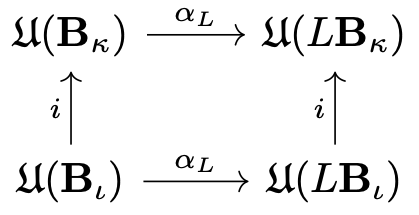
\[\begin{align} \alpha_L : \mathfrak{U}(\mathbf{B}) &\longrightarrow \mathfrak{U}(L\mathbf{B}) \\ a &\longmapsto \alpha_L(a) \end{align}\]where \(L\mathbf{B}\) is the image of the region \(\mathbf{B}\) under the transformation \(L\) and \(\alpha_L\) is a unital *-isomorphism generated by \(L\). The map \(\alpha_L\) is such that (1) for the identity element \(\mathbf{1}\) of the Lorentz group it satisfies
\[\alpha_{\mathbf{1}}(a) = a,\](2) for all appropriate \(a\), \(L\), and \(L'\) it satisfies
\[\alpha_{L' \cdot L}(a) = \alpha_{L'}(\alpha_{L}(a)),\]and (3) for basis elements \(\mathbf{B}_\iota \subset \mathbf{B}_\kappa\) and the unital *-monomorphism \(i\) of Axiom 2 (Isotony) \(\alpha_L\) commutes with \(i\). In other words the following diagram
commutes.
This concludes the presentation of the “sharpened” axioms. As proven in this blog post, these “sharpened” axioms entail the original axioms save Axiom 6 (Primitivity), which is an axiom that we abandon.
These “sharpened” axioms also allow for a straightforward generalization to a set of axioms describing AQFT in curved spacetime, i.e. a set of axioms describing AQFT in a curved spacetime background that is fixed and treated classically. In a subsequent blog post we will detail these axioms.
The notation \(a_R\) used here is used instead of the more traditional \(\pi_\omega(a)\) to prevent a degression into the GNS construction, which we none-the-less present later. ↩
Technically, one only requires the existence of a “bounded, approximate identity” and not a unit to produce a distinguished vector \(\Omega_\omega\). However, physical motivation for the existence of a “bounded, approximate identity” as opposed to a unit is lacking. ↩
Given \(\mathcal{N}\) a self-adjoint subset of \(\mathcal{B}(\mathcal{H}_\omega)\) the set of bounded operators on \(\mathcal{H}_\omega\) ( i.e. \(\mathcal{N} \subseteq \mathcal{B}(\mathcal{H}_\omega)\) such that \(\mathcal{N}^*=\mathcal{N}\) ) we define \(\mathcal{N}' \equiv \{ N' \in \mathcal{B}(\mathcal{H}_\omega) : NN' - N'N = 0 \; \forall N \in \mathcal{N} \}\) and similarly define the shorthand \(\mathcal{N}'' \equiv (\mathcal{N}')'\). ↩
Again, technically, one only requires the existence of a “bounded, approximate identity” and not a unit to produce a distinguished vector \(\Omega_\omega\). However, physical motivation for the existence of a “bounded, approximate identity” as opposed to a unit is lacking. ↩
The universal representation of a unital C*-algebra is the direct sum of all of its representations created via the GNS construction. ↩