This blog post presents the axioms governing Algebraic Quantum Field Theory (AQFT) in curved spacetime, generalizing the axioms of AQFT in Minkowski spacetime from the blog post Unpacking the Haag Kastler Axioms.

As in Unpacking the Haag Kastler Axioms, we aim to “simplify” the axioms. Also, in contrast to the standard presentation of AQFT in curved spacetime (i.e. Locally Covariant Quantum Field Theory (LCQFT) of Brunetti, Fredenhagen, and Verch), here we require no category theory and thus retain more of a physics “feel”.

Haag Kastler Axioms in Minkowski Spacetime

Before jumping directly into AQFT in curved spacetime, this section takes a moment to review AQFT in Minkowski spacetime. This review generally distills the presentation of Unpacking the Haag Kastler Axioms.

Prologue

Generally AQFT is thought to “unfold” on “Minkowski spacetime”. However, most AQFT presentations spend little to no time detailing exactly what “Minkowski spacetime” is. It’s regarded as being too “basic”.

None-the-less, we dedicate this section to reviewing “Minkowski spacetime”. This pedantic review will bear later fruit, as understanding the subtleties of “Minkowski spacetime” will greatly aid in understanding the subtleties of AQFT on “Minkowski spacetime”.

Smooth Manifold

As a set “Minskowski spacetime” is \(\mathbb{R}^4\). This set is then equipped with the Euclidean topology by: (1) equipping \(\mathbb{R}^4\) with the Euclidean norm, (2) defining a Euclidean metric on \(\mathbb{R}^4\) using this Euclidean norm, and (3) defining the Euclidean topology as the topology generated by the open balls of this Euclidean metric. The set \(\mathbb{R}^4\) equipped with this Euclidean topology makes \(\mathbb{R}^4\) a topological manifold.

For a generic topological manifold \(M\) one defines a chart as a pair \((U,\varphi_U)\) in which \(U\) is an open set of \(M\) and \(\varphi_U : U \rightarrow \widehat{U}\) is a homeomorphism from \(U\) to the open set \(\widehat{U} \equiv \varphi_U(U)\) of \(\mathbb{R}^n\). (Note, here \(\mathbb{R}^n\) is equipped with the Euclidean topology.) If one has a pair of charts \((U,\varphi_U)\) and \((V,\varphi_V)\) on \(M\), then the map

is called a transition map. The charts \((U,\varphi_U)\) and \((V,\varphi_V)\) are said to be smoothly compatible if \(U \cap V\) is the empty set or the transition map \(\varphi_V \circ \varphi_U^{-1}\) is a diffeomorphism. (\(\varphi_V \circ \varphi_U^{-1}\) is a map from an open subset of \(\mathbb{R}^4\) to an open subset of \(\mathbb{R}^4\). So this is well-defined.)

An atlas for \(M\) is a set of charts whose domains cover all of \(M\). A smooth atlas on \(M\) is an atlas in which any two charts are smoothly compatible. Such a smooth atlas is maximal if it is not the proper subset of any other smooth atlas. Finally, a smooth structure on \(M\) is a maximal smooth atlas on \(M\), and the topological manifold \(M\) is in addition a smooth manifold if admits a smooth structure.

As is relatively obvious, \(\mathbb{R}^4\) equipped with the Euclidean topology is a smooth manifold. The charts of the maximal smooth atlas on \(\mathbb{R}^4\) are simply pairs of the form \((U, \varphi)\), where \(U\) is an open set of the Euclidean topology and \(\varphi\) is a diffeomorphism. So, \(\mathbb{R}^4\), which will form the “core” of “Minkowski spacetime”, is a smooth manifold.

Existence of a Minkowski Metric

We’ve established that \(\mathbb{R}^4\) equipped with the Euclidean topology is a smooth manifold, and we’ve also defined a Euclidean metric on \(\mathbb{R}^4\). What we have not yet done is defined a Minkowski metric on \(\mathbb{R}^4\). It is to this we now turn.

One might hope that one could simply place a Minkowski metric on \(\mathbb{R}^4\) without any additional structure. However, this is not the case. “Morally” the reason for this is that at each point a Minkowski metric, which is a type of Lorentz metric, “distinguishes” a “time direction” from all other directions. So, one might guess that to specify a Minkowski metric one would have to specify a distinguished “time” direction at each point. It turns out that this is indeed the case.

The following theorem (Theorem 2.69 from Lee)

Theorem (Existence of a Lorentz Metric) A smooth manifold \(M\) admits a smooth Lorentz metric if and only if it admits a smooth, global vector field.

governs when a Lorentz, and thus Minkowski metric exists. As expected, it requires the existence of a smooth, global vector field that at each point specifies a distinguished “time” direction.

So in order to introduce a Minkowski metric on \(\mathbb{R}^4\), we must first introduce a smooth, global vector field on \(\mathbb{R}^4\). Traditionally this smooth, global vector field is taken to be \(t^\mu \equiv (1,0,0,0)\) in the standard global coordinates on \(\mathbb{R}^4\). This can then be used to derive the standard Minkowski metric on \(\mathbb{R}^4\).

Alexandrov Topology

With the smooth manifold \(\mathbb{R}^4\) equipped with a smooth, global vector field \(t^a\) and a Minkowski metric, one might think we’ve completed the construction of “Minkowski spacetime”. In most treatments of “Minkowski spacetime”, this is indeed where the presentation ends. We won’t end here, but instead add another level of detail pertinent to AQFT on “Minkowski spacetime”.

To wit, what might seem “odd” about the construction to this point is the central role played by the Euclidean norm, Euclidean metric, and Euclidean topology. The entire construction starts by placing a Euclidean norm on \(\mathbb{R}^4\), then using this norm to define a Euclidean metric on \(\mathbb{R}^4\) which in turn is used to define the Euclidean topology.

Physics relies upon a Minkowski metric not a Euclidean metric. Why does one have to make such “heavy” use of the Euclidean norm, Euclidean metric, and Euclidean topology? “Morally” they should have nothing to do with physics.

“Morally” the entire development should only rely upon “Minkowski” constructions. We should be able to introduce a “Minkowski topology” and jettison the Euclidean topology. But the question is what does a “Minkowski topology” even mean?

To consider what that might mean, let \(p\) and \(q\) be any two points in \(\mathbb{R}^4\). With these two points, we can define two sets: \(I^+(p)\), the chronological future of \(p\) (i.e. the set of points reachable from \(p\) via a future-directed, time-like curve), and \(I^-(q)\), the chronological past of \(q\) (i.e. the set of all points that reach \(q\) via a future-directed, time-like curve).

It turns out that \(I^+(p)\) is an open set in the Euclidean topology for any \(p\) (Proposition 2.8 of Penrose). Similarly, the time-reversed version of Proposition 2.8 of Penrose implies that \(I^-(q)\) is an open set in that same topology. Hence, \(I^+(p) \cap I^-(q)\) is open in the Euclidean topology.

This suggests that sets of the form \(I^+(p) \cap I^-(q)\) might be able to be used as the basis of a new topology on \(\mathbb{R}^4\). As it so happens, sets of this form can be used as the basis for a topology on \(\mathbb{R}^4\).

Sets \(I^+(p) \cap I^-(q)\) with \(p,q \in \mathbb{R}^4\) form the basis for what’s known as the Alexandrov topology of \(\mathbb{R}^4\) (Definition 4.22 of Penrose). (This is also sometimes known as the interval topology of \(\mathbb{R}^4\) (Remark 4.23 of Penrose).) Furthermore, it turns out that the Alexandrov topology of \(\mathbb{R}^4\) agrees with the Euclidean topology of \(\mathbb{R}^4\) (Paragraph 4.23 of Penrose), a welcome happenstance that “explains” why physicists had not confronted this earlier.

Minkowski Spacetime

Now with the introduction of the Alexandrov topology, we can finally define “Minkowski spacetime”. For us Minkowski spacetime is the smooth manifold \(\mathbb{R}^4\) equipped with a smooth, global vector field \(t^a\) and a Minkowski metric, where the topology of \(\mathbb{R}^4\) is the Alexandrov topology and not the Euclidean topology.

This results in Minkowski spacetime being “clearly physical”, in that it doesn’t rely upon a Euclidean norm, metric, or topology. Furthermore, as the Alexandrov topology agrees with the Euclidean topology (Paragraph 4.23 of Penrose), Minkowski spacetime doesn’t rely upon the Euclidean “scaffolding” we used to construct it.

Axiom 1 (Local Algebras)

With this prologue completed, we are now able to state the first axiom of AQFT in Minkowski spacetime:

Axiom 1 (Local Algebras) For any basis element \(\mathbf{B}\) of the Alexandrov topology on Minkowski spacetime, i.e. any set of the form \(I^+(p) \cap I^-(q)\), there is a corresponding abstract C*-algebra \(\mathfrak{U}(\mathbf{B})\)

\[\mathbf{B} \longmapsto \mathfrak{U}(\mathbf{B}),\]

and when \(\mathbf{B}\) is the the empty set, we have the distinguished correspondence

\[\emptyset \longmapsto \mathbb{C} \mathbf{1},\]

where \(\mathbf{1}\) is the multiplicative identity in the C*-algebra \(\mathbb{C} \mathbf{1}\).

Axiom 2 (Isotony)

The second axiom takes the following form:

Axiom 2 (Isotony) Let \(\mathbf{B}_1\) and \(\mathbf{B}_2\) be any two basis elements of the Alexandrov topology on Minkowski spacetime, i.e. any two sets of the form \(I^+(p_1) \cap I^-(q_1)\) and \(I^+(p_2) \cap I^-(q_2)\).

If \(\mathbf{B}_1 \subset \mathbf{B}_2\) then \(\mathfrak{U}(\mathbf{B}_1) \subset \mathfrak{U}(\mathbf{B}_2)\), where inclusion is implemented by

\[i : \mathfrak{U}(\mathbf{B}_1) \hookrightarrow \mathfrak{U}(\mathbf{B}_2),\]

a unital *-homomorphism.

Axiom 3 (Local Commutativity)

Before stating the next axiom, we need to introduce some terminology that will aid in stating the axiom.

Definition (Quasilocal Algebra) Consider the set-theoretic union of all \(\mathfrak{U}(\mathbf{B})\). As proven in the previous blog post (Unpacking the Haag Kastler Axioms), this set-theoretic union is a normed *-algebra. Also, as proven in the previous blog post (Unpacking the Haag Kastler Axioms), its completion yields a C*-algebra, denoted as \(\mathfrak{U}\). This C*-algebra \(\mathfrak{U}\) is called the quasilocal algebra.

Definition (Causal Future and Past) Consider a point \(p\) in Minkowski spacetime. The causal future of \(p\) is the set \(J^+(p)\) of points reachable from \(p\) via a future-directed, time-like or light-like curve. Similarly, the causal past of \(p\) is the set \(J^-(p)\) of all points that reach \(p\) via a future-directed, time-like or light-like curve.

Definition (Spacelike Related) Consider two points \(p_1\) and \(p_2\) in Minkowski spacetime. The points are said to be spacelike related if \(p_2 \notin J^+(p_1) \cup J^-(p_1)\) or equivalently \(p_1 \notin J^+(p_2) \cup J^-(p_2)\).

Definition (Completely Spacelike) Consider two sets \(\mathbf{O}_1\) and \(\mathbf{O}_2\) in Minkowski spacetime. \(\mathbf{O}_1\) and \(\mathbf{O}_2\) are said to be completely spacelike if every \(p_1\) in \(\mathbf{O}_1\) is spacelike related to every \(p_2\) in \(\mathbf{O}_2\) or equivalently if every \(p_2\) in \(\mathbf{O}_2\) is spacelike related to every \(p_1\) in \(\mathbf{O}_1\).

With all of these definitions in hand, we can now state the next axiom:

Axiom 3 (Local Commutativity) Let \(\mathbf{B}_1\) and \(\mathbf{B}_2\) be any two basis elements of the Alexandrov topology on Minkowski spacetime, i.e. any two sets of the form \(I^+(p_1) \cap I^-(q_1)\) and \(I^+(p_2) \cap I^-(q_2)\).

If \(\mathbf{B_1}\) and \(\mathbf{B_2}\) are completely spacelike, then \(\mathfrak{U}(\mathbf{B_1})\) and \(\mathfrak{U}(\mathbf{B_2})\) commute in the quasilocal algebra \(\mathfrak{U}\), i.e. for any \(a_1\) in \(\mathfrak{U}(\mathbf{B_1})\) and \(a_2\) in \(\mathfrak{U}(\mathbf{B_2})\) it follows that

\[a_1 a_2 - a_2 a_1 = 0\]

in the quasilocal algebra \(\mathfrak{U}\).

Axiom 4 (Quasilocal Algebra)

To state the next axiom we make use of the following definition which relies upon some constructs presented in the previous blog post (Unpacking the Haag Kastler Axioms).

Definition (Quasilocal Observable) The image \(\pi_\omega(a)\) of a self-adjoint member \(a\) of the quasilocal algebra \(\mathfrak{U}\) under a GNS *-homomorphism \(\pi_\omega\) of state \(\omega\) is self-adjoint and thus corresponds to an “observable”. Any “observable” corresponding to such a self-adjoint \(\pi_\omega(a)\) is called a quasilocal observable.

Using this definition we can then state the next axiom

Axiom 4 (Quasilocal Algebra) All “observables” are quasilocal observables.

Axiom 5 (Lorentz Covariance)

Finally we can state the last axiom

Axiom 5 (Lorentz Covariance) Let \(\mathbf{B}\) be any basis element of the Alexandrov topology on Minkowski spacetime, i.e. any set of the form \(I^+(p) \cap I^-(q)\).

A member \(L\) of the inhomogeneous Lorentz group homotopic to the identity acts on a \(\mathfrak{U}(\mathbf{B}) \subset \mathfrak{U}\) as follows

\[\mathfrak{U}(\mathbf{B}) \longmapsto \mathfrak{U}(\mathbf{LB}),\]

where \(L\mathbf{B}\) is the image of the basis element \(\mathbf{B}\) under the transformation \(L\).

Haag Kastler Axioms in Curved Spacetime

As we’ve recounted the axioms of AQFT in Minkowski spacetime, we are now in a position to generalize this to curved spacetime, i.e. “Lorentzian spacetime”. Surprisingly the generalization to “Lorentzian spacetime” is relatively straightforward.

We note, however, that as in the case of AQFT in Minkowski spacetime, the generalization to “Lorentzian spacetime” will not account for “backreaction” of the quantum fields on “Lorentzian spacetime”. The “Lorentzian spacetime” will be a fixed, classical background upon which AQFT “unfolds”.

Prologue

Most presentations of AQFT in curved spacetime gloss over the details of exactly what “Lorentzian spacetime” is. It’s too “basic”.

In contrast to those presentations, we want to spend some time detailing exactly what “Lorentzian spacetime” is before we formulate AQFT there. This level of pedantry will serve us well when formulating AQFT on “Lorentzian spacetime”, helping to motivate otherwise opaque aspects of the formulation.

Smooth Manifold

Consider a smooth, connected, four dimensional Hausdorff manifold \(M\) equipped with a topology, which we simply call the “manifold topology”. This will form the “core” of our definition of a “Lorentzian spacetime”.

Existence of a Lorentzian Metric

As we wish this \(M\) to be a “Lorentzian spacetime”, it should support a Lorentzian metric. Not all such \(M\) support Lorentzian metrics. In fact for such an \(M\) to support a Lorentzian metric, it must admit additional structure.

In particular, as we have seen previously, the required structure follows from the theorem (Theorem 2.69 from Lee)

Theorem (Existence of a Lorentz Metric) A smooth manifold \(M\) admits a smooth Lorentz metric if and only if it admits a smooth, global vector field.

So, we require, in addition to all the structure \(M\) already supports, that it also supports a smooth, global vector field \(t^a\), as this is required for \(M\) to support a smooth Lorentzian metric.

Alexandrov Topology

As in the case of a Minkowski spacetime, it’s “odd” that the manifold topology on \(M\) may have nothing to do with the Lorentzian nature of spacetime. The manifold topology could, as was the case for Minkowski spacetime, be derived from purely Euclidean metrics. Physics isn’t Euclidean; so there seems to be a fundamental tension.

In the case of Minkowski spacetime we introduced sets of the form \(I^+(p) \cap I^-(q)\), showed that they are open in the Euclidean topology (Proposition 2.8 of Penrose), and can be used as the basis of the Alexandrov topology (Definition 4.22 of Penrose). Furthermore, we showed that the Alexandrov topology is equivalent to the Euclidean topology (Paragraph 4.23 of Penrose). We want to generalize all of this to “Lorentzian spacetimes”.

It turns out that just as in the case of Minkowski spacetime, sets of the form \(I^+(p) \cap I^-(q)\) on \(M\) are open sets in the manifold topology (Proposition 2.8 of Penrose). Furthermore, on \(M\) they also form the basis of a topology (Definition 4.22 of Penrose), again called the Alexandrov topology. However, for \(M\) the relationship between the Alexandrov topology and the manifold topology is more nuanced than in the case of Minkowski spacetime.

It turns out that to understand this nuance, we need to introduce several definitions that aid in the process.

Definition (Causally Convex) Consider an open subset \(\mathbf{O}\) of a smooth, connected, four dimensional Hausdorff manifold \(M\) that is equipped with a Lorentzian metric. \(\mathbf{O}\) is said to be causally convex if for every \(p\) and \(r\) in \(\mathbf{O}\) and \(q\) in \(M\) the existence of a future-directed, time-like curve from \(p\) to \(q\) and a future-directed, time-like curve from \(q\) to \(r\) implies that \(q\) is a member of \(\mathbf{O}\).

Definition (Strongly Causal) Consider a smooth, connected, four dimensional Hausdorff manifold \(M\) that is equipped with a Lorentzian metric. \(M\) is said to be strongly causal at \(p \in M\) if \(p\) has arbitrarily small causally convex neighborhoods. \(M\) is said to be strongly causal if \(M\) is strongly causal at every \(p \in M\).

With these definitions in hand we can then present the key theorem describing how the Alexandrov topology and the manifold topology are related (Theorem 4.24 of Penrose):

Theorem (Properties of the Alexandrov Topology) The following three conditions on a smooth, connected, four dimensional manifold \(M\) with Hausdorff manifold topology are equivalent:

1. \(M\) is strongly causal;
2. the Alexandrov Topology agrees with the manifold topology;
3. the Alexandrov Topology is Hausdorff.

As one can see, this has “deep” implications for the case at hand, the smooth manifold \(M\).

Physically, the Alexandrov topology seems more “natural” as it relies upon basis elements \(I^+(p) \cap I^-(q)\) “natural” to Lorentzian nature of spacetime. So physically one would expect a “Lorentzian spacetime” to “naturally” be equipped with an Alexandrov topology. The question is how does one accomplish this goal?

In the case of Minkowski spacetime the Alexandrov topology on \(\mathbb{R}^4\) agreed with the Euclidean topology without any further assumptions. The Euclidean “scaffolding” used to construct the Alexandrov topology simply “fell away”. The previous theorem implies that for the more general case we are dealing with now on \(M\), removing the manifold topology “scaffolding” requires additional assumptions.

In particular, we can either assume that \(M\) is strongly causal or that the Alexandrov Topology is Hausdorff. Either assumption implies the other and that the Alexandrov Topology agrees with the manifold topology, and thus the manifold topology “scaffolding” can be removed.

As both assumptions are equivalent, we can select either. With that in mind, we add the additional assumption that the Alexandrov Topology on \(M\) is Hausdorff. So in total \(M\) is a smooth, connected, four dimensional manifold equipped with a Hausdorff Alexandrov topology. In addition \(M\) is equipped with a smooth, global vector field \(t^a\) and associated Lorentzian metric.

Lorentzian Spacetime

Finally we have all the pieces in place to define a “Lorentzian spacetime”.

Definition (Lorentzian Spacetime) A Lorentzian spacetime is a smooth, connected, four dimensional manifold equipped with a Hausdorff Alexandrov topology. In addition it is equipped with a smooth, global vector field \(t^a\) and associated Lorentzian metric.

It will be on such Lorentzian spacetimes that AQFT “unfolds”.

Axiom 1 (Local Algebras)

With the prologue complete, we are now in a position to state the axioms of AQFT on Lorentzian spacetime. Surprisingly, all the hard work is done.

The first axiom is:

Axiom 1 (Local Algebras) For any basis element \(\mathbf{B}\) of the Alexandrov topology on a Lorentzian spacetime, i.e. any set of the form \(I^+(p) \cap I^-(q)\), there is a corresponding abstract C*-algebra \(\mathfrak{U}(\mathbf{B})\)

\[\mathbf{B} \longmapsto \mathfrak{U}(\mathbf{B}),\]

and when \(\mathbf{B}\) is the the empty set, we have the distinguished correspondence

\[\emptyset \longmapsto \mathbb{C} \mathbf{1},\]

where \(\mathbf{1}\) is the multiplicative identity in the C*-algebra \(\mathbb{C} \mathbf{1}\).

Axiom 2 (Isotony)

The second axiom takes the following form:

Axiom 2 (Isotony) Let \(\mathbf{B}_1\) and \(\mathbf{B}_2\) be any two basis elements of the Alexandrov topology on a Lorentzian spacetime, i.e. any two sets of the form \(I^+(p_1) \cap I^-(q_1)\) and \(I^+(p_2) \cap I^-(q_2)\).

If \(\mathbf{B}_1 \subset \mathbf{B}_2\) then \(\mathfrak{U}(\mathbf{B}_1) \subset \mathfrak{U}(\mathbf{B}_2)\), where inclusion is implemented by

\[i : \mathfrak{U}(\mathbf{B}_1) \hookrightarrow \mathfrak{U}(\mathbf{B}_2),\]

a unital *-homomorphism.

Axiom 3 (Local Commutativity)

So far the axioms have differed little from those of AQFT in Minkowski spacetime. This ceases to be true for subsequent axioms. The primary reason for this is that the existence of a quasilocal algebra is not guaranteed on a Lorentzian spacetime. Let us prove this is the case.

Quasilocal Algebra?

Naively, to define a quasilocal algebra associated with a Lorentzian spacetime \(M\) one would first consider the set-theoretic union of all \(\mathfrak{U}(\mathbf{B})\) over all basis elements \(\mathbf{B}\) of the Alexandrov topology on \(M\) and prove this set-theoretic union is a normed *-algebra. It turns out that for a generic Lorentzian spacetime \(M\) this set-theoretic union isn’t a normed *-algebra and thus the construction of the quasilocal algebra fails. Let’s see why this is the case.

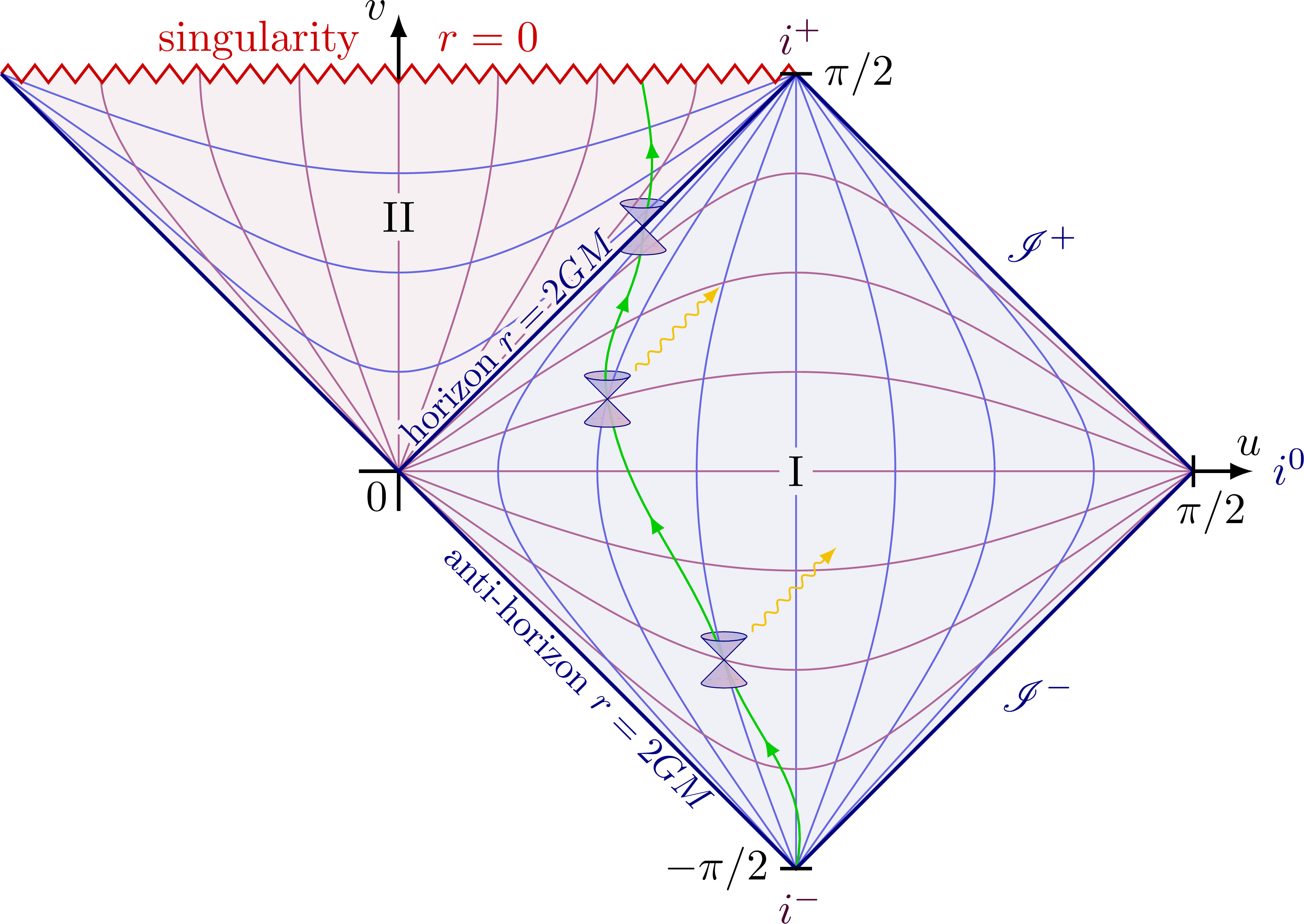
Consider \(M_{BH}\) the Schwarzschild blackhole solution Lorentzian spacetime. \(M_{BH}\) has the following Penrose diagram

Zooming in on the singularity we can introduce two basis elements \(\mathbf{B}_1\) and \(\mathbf{B}_2\) of the Alexandrov topology that are \(\varepsilon\) from the singularity

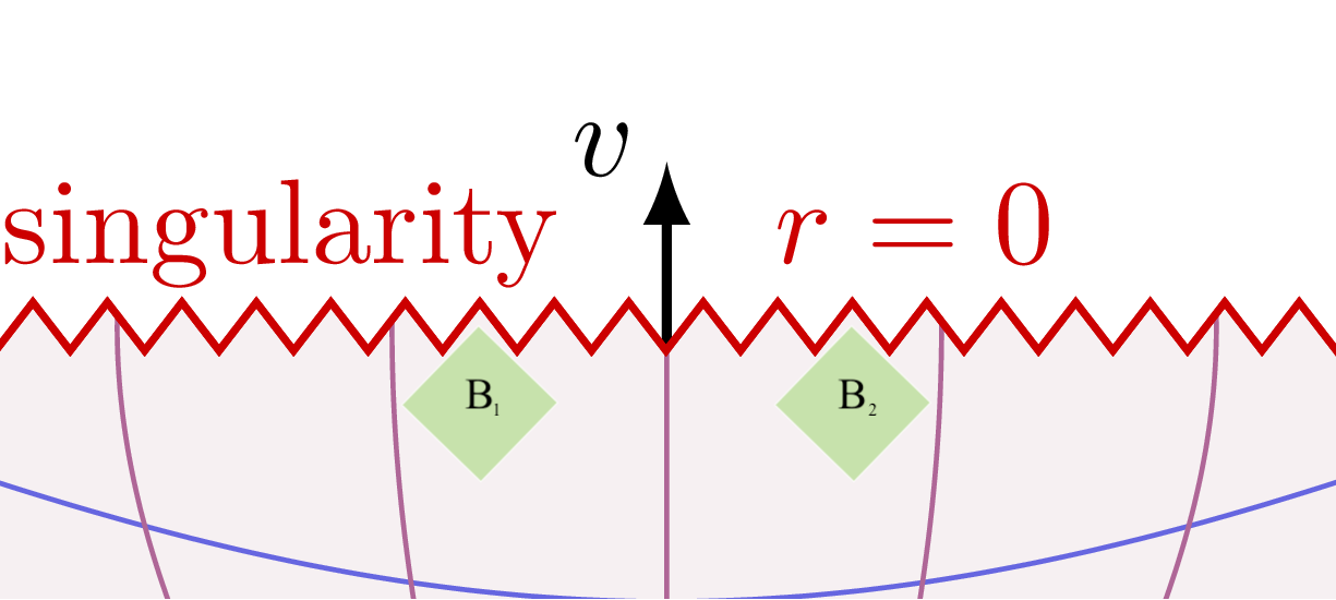
What is obvious is that there exists no basis element \(\mathbf{B}\) of the Alexandrov topology that contains both \(\mathbf{B}_1\) and \(\mathbf{B}_2\) as it would have to extend beyond the singularity off of \(M_{BH}\)

which is of course not allowed.

As a result of this, one can not employ the isotony axiom, the only tool one has, to place \(\mathfrak{U}(\mathbf{B}_1)\) and \(\mathfrak{U}(\mathbf{B}_2)\) in a larger algebra, an algebra in which addition and multiplication of their elements would make sense.

This implies that the set-theoretic union of all \(\mathfrak{U}(\mathbf{B})\) over all basis elements \(\mathbf{B}\) of the Alexandrov topology on \(M_{BH}\) is not a normed *-algebra. This in turn implies that the construction of the quasilocal algebra fails¹ for \(M_{BH}\).

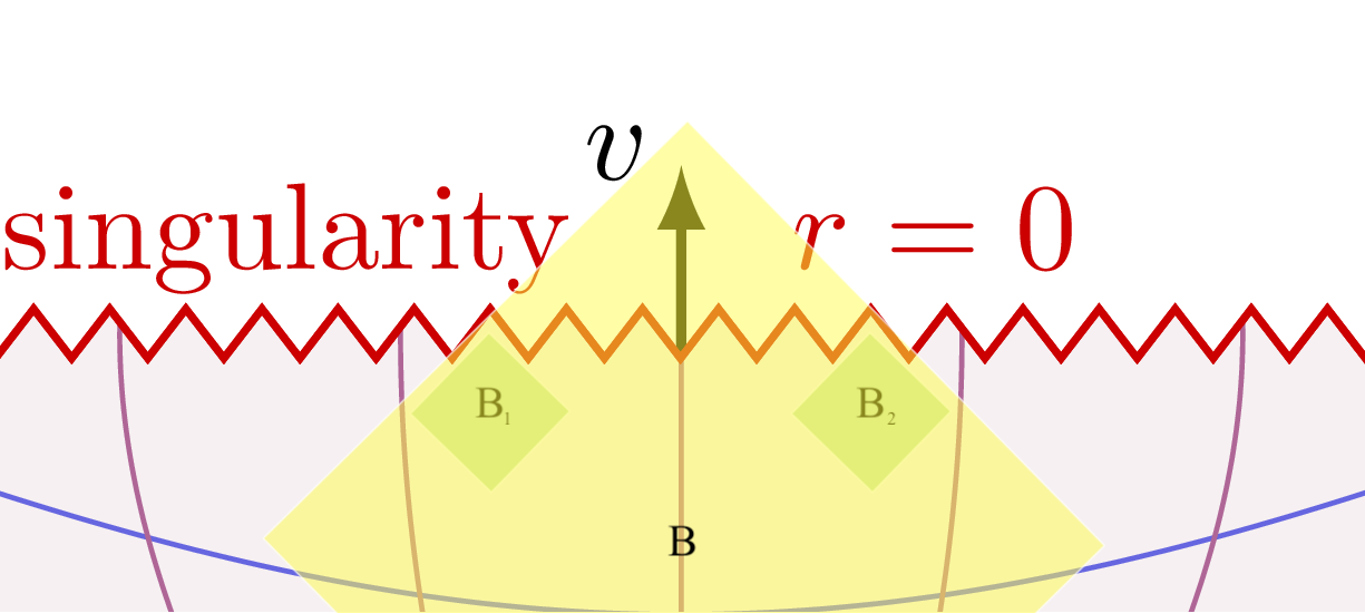
For any two basis elements \(\mathbf{B}_1\) and \(\mathbf{B}_2\) of the Alexandrov topology on a generic Lorentzian spacetime \(M\) the best one can hope for is that there exists a third element \(\mathbf{B}\) of the Alexandrov topology such that \(\mathbf{B}_1, \mathbf{B}_2 \subseteq \mathbf{B}\). However, there is no guarantee that such a \(\mathbf{B}\) exists in a Lorentzian spacetime.

All that being said, we can still state a variation of Axiom 3 (Local Commutativity) that applies to a Lorentzian spacetime. But before doing so we have to introduce some terminology.

Causality and Chronology

As in the case of AQFT on Minkowski spacetime, we have to introduce a few definitions related to causality and chronology. Thankfully, they are the obvious variations of those that applied to Minkowski spacetime.

Definition (Causal Future and Past) Consider a point \(p\) in Lorentzian spacetime. The causal future of \(p\) is the set \(J^+(p)\) of points reachable from \(p\) via a future-directed, time-like or light-like curve. Similarly, the causal past of \(p\) is the set \(J^-(p)\) of all points that reach \(p\) via a future-directed, time-like or light-like curve.

Definition (Spacelike Related) Consider two points \(p_1\) and \(p_2\) in Lorentzian spacetime. The points are said to be spacelike related if \(p_2 \notin J^+(p_1) \cup J^-(p_1)\) or equivalently \(p_1 \notin J^+(p_2) \cup J^-(p_2)\).

Definition (Completely Spacelike) Consider two sets \(\mathbf{O}_1\) and \(\mathbf{O}_2\) in Lorentzian spacetime. \(\mathbf{O}_1\) and \(\mathbf{O}_2\) are said to be completely spacelike if every \(p_1\) in \(\mathbf{O}_1\) is spacelike related to every \(p_2\) in \(\mathbf{O}_2\) or equivalently if every \(p_2\) in \(\mathbf{O}_2\) is spacelike related to every \(p_1\) in \(\mathbf{O}_1\).

Axiom 3 (Local Commutativity)

With all of these definitions in hand, we can finally state Axiom 3 (Local Commutativity) as applied to Lorentzian spacetime:

Axiom 3 (Local Commutativity) Let \(\mathbf{B}_1\) and \(\mathbf{B}_2\) be any two basis elements of the Alexandrov topology on Lorentzian spacetime, i.e. any two sets of the form \(I^+(p_1) \cap I^-(q_1)\) and \(I^+(p_2) \cap I^-(q_2)\).

If \(\mathbf{B_1}\) and \(\mathbf{B_2}\) are completely spacelike and there exists a basis element \(\mathbf{B}\) such that \(\mathbf{B_1}, \mathbf{B_2} \subseteq \mathbf{B}\) then \(\mathfrak{U}(\mathbf{B_1})\) and \(\mathfrak{U}(\mathbf{B_2})\) commute in the C*-algebra \(\mathfrak{U}(\mathbf{B})\), i.e. for any \(a_1\) in \(\mathfrak{U}(\mathbf{B_1})\) and \(a_2\) in \(\mathfrak{U}(\mathbf{B_2})\) it follows that

\[a_1 a_2 - a_2 a_1 = 0\]

in the C*-algebra \(\mathfrak{U}(\mathbf{B})\).

If no such \(\mathbf{B}\) exists, then it simply doesn’t make sense to consider if \(\mathfrak{U}(\mathbf{B_1})\) and \(\mathfrak{U}(\mathbf{B_2})\) commute as they are not in the same algebra.

While having the commutation status of \(\mathfrak{U}(\mathbf{B_1})\) and \(\mathfrak{U}(\mathbf{B_2})\) sometimes being undefined seems “odd” at first. It’s actually not “odd” at all. The commutation status of \(\mathfrak{U}(\mathbf{B_1})\) and \(\mathfrak{U}(\mathbf{B_2})\) is only undefined when it’s impossible to conduct an experiment that determines if they commute. This makes complete sense.

Axiom 4 (Local Algebra)

The axiom we are about to present also changes slightly from its analog Axiom 4 (Quasilocal Algebra) on Minkowski spacetime. The reason for the change, as was the reason for the change in Axiom 3 (Local Commutativity), is the fact that there is no such thing as a quasilocal algebra on a generic Lorentzian spacetime.

Before we state the next axiom for Lorentzian spacetimes, we need to, as in the case of Minkowski spacetime, present a definition used in the statement of the axiom.

This definition relies upon the fact, which one may check, that the GNS construction for a state \(\omega\) on a C*-algebra \(\mathfrak{U}(\mathbf{B})\), where \(\mathbf{B}\) is an element of the Alexandrov topology on the Lorentzian spacetime \(M\), works just as described in the previous blog post (Unpacking the Haag Kastler Axioms).

Definition (Local Observable) For Lorentzian spacetime \(M\) the image \(\pi_\omega(a)\) of a self-adjoint member \(a\) of the local algebra \(\mathfrak{U}(\mathbf{B})\) under the GNS *-homomorphism \(\pi_\omega\) of a state \(\omega\) on \(\mathfrak{U}(\mathbf{B})\) is self-adjoint and thus corresponds to an “observable”. Any “observable” corresponding to such a self-adjoint \(\pi_\omega(a)\) is called a local observable.

Using this definition we can state the axiom

Axiom 4 (Local Algebra) All “observables” are local observables.

As shown in the blog post Unpacking the Haag Kastler Axioms, this axiom is essentially the statement that there exist “observables” that are not local observables, but such “observables” are “experimentally indistinguishable” from local observables and thus can be ignored.

Axiom 5 (General Covariance)

Now we present the final, and most interesting, axiom in the case of Lorentzian spacetimes.

The interesting aspect of this theorem is understanding what replaces the inhomogeneous Lorentz group homotopic to the identity, which appears in the Minkowski spacetime analog. One might think to replace it with diffeomorphisms of a Lorentzian spacetime. However, this isn’t the correct analog.

Lorentzian spacetimes can admit diffeomorphisms that are not homotopic to the identity. (For example, in two dimensions Dehn twists aren’t homotopic to the identity.) So, if we want to “mirror” Axiom 5 (Lorentz Covariance) from the Minkowski case (which only considers group elements homotopic to the identity), we should limit the diffeomorphisms we employ.

The “natural” choice seems to be the set of diffeomorphisms that are homotopic to the identity. Using this, the axiom takes the following form:

Axiom 5 (General Covariance) Let \(\mathbf{B}\) be any basis element of the Alexandrov topology on a Lorentzian spacetime \(M\), i.e. any set of the form \(I^+(p) \cap I^-(q)\).

A member \(\varphi\) of the group of diffeomorphisms of \(M\) that are homotopic to the identity acts on \(\mathfrak{U}(\mathbf{B})\) as follows

\[\mathfrak{U}(\mathbf{B}) \longmapsto \mathfrak{U}(\varphi(\mathbf{B})),\]

where \(\varphi(\mathbf{B})\) is the image of the basis element \(\mathbf{B}\) under the diffeomorphism \(\varphi\).

Summary

Here we recount the axioms we’ve established for AQFT in Lorentzian spacetime.

First we remind the reader of the Lorentzian spacetime definition

Definition (Lorentzian Spacetime) A Lorentzian spacetime is a smooth, connected, four dimensional manifold equipped with a Hausdorff Alexandrov topology. In addition it is equipped with a smooth, global vector field \(t^a\) and associated Lorentzian metric.

With that clarified, we can present the first axiom

Axiom 1 (Local Algebras) For any basis element \(\mathbf{B}\) of the Alexandrov topology on a Lorentzian spacetime, i.e. any set of the form \(I^+(p) \cap I^-(q)\), there is a corresponding abstract C*-algebra \(\mathfrak{U}(\mathbf{B})\)

\[\mathbf{B} \longmapsto \mathfrak{U}(\mathbf{B}),\]

and when \(\mathbf{B}\) is the the empty set, we have the distinguished correspondence

\[\emptyset \longmapsto \mathbb{C} \mathbf{1},\]

where \(\mathbf{1}\) is the multiplicative identity in the C*-algebra \(\mathbb{C} \mathbf{1}\).

The second axiom can be immediately stated too.

Axiom 2 (Isotony) Let \(\mathbf{B}_1\) and \(\mathbf{B}_2\) be any two basis elements of the Alexandrov topology on a Lorentzian spacetime, i.e. any two sets of the form \(I^+(p_1) \cap I^-(q_1)\) and \(I^+(p_2) \cap I^-(q_2)\).

If \(\mathbf{B}_1 \subset \mathbf{B}_2\) then \(\mathfrak{U}(\mathbf{B}_1) \subset \mathfrak{U}(\mathbf{B}_2)\), where inclusion is implemented by

\[i : \mathfrak{U}(\mathbf{B}_1) \hookrightarrow \mathfrak{U}(\mathbf{B}_2),\]

a unital *-homomorphism.

The next axiom makes use of the following definitions:

Definition (Causal Future and Past) Consider a point \(p\) in Lorentzian spacetime. The causal future of \(p\) is the set \(J^+(p)\) of points reachable from \(p\) via a future-directed, time-like or light-like curve. Similarly, the causal past of \(p\) is the set \(J^-(p)\) of all points that reach \(p\) via a future-directed, time-like or light-like curve.

Definition (Spacelike Related) Consider two points \(p_1\) and \(p_2\) in Lorentzian spacetime. The points are said to be spacelike related if \(p_2 \notin J^+(p_1) \cup J^-(p_1)\) or equivalently \(p_1 \notin J^+(p_2) \cup J^-(p_2)\).

Definition (Completely Spacelike) Consider two sets \(\mathbf{O}_1\) and \(\mathbf{O}_2\) in Lorentzian spacetime. \(\mathbf{O}_1\) and \(\mathbf{O}_2\) are said to be completely spacelike if every \(p_1\) in \(\mathbf{O}_1\) is spacelike related to every \(p_2\) in \(\mathbf{O}_2\) or equivalently if every \(p_2\) in \(\mathbf{O}_2\) is spacelike related to every \(p_1\) in \(\mathbf{O}_1\).

and can be stated as follows:

Axiom 3 (Local Commutativity) Let \(\mathbf{B}_1\) and \(\mathbf{B}_2\) be any two basis elements of the Alexandrov topology on Lorentzian spacetime, i.e. any two sets of the form \(I^+(p_1) \cap I^-(q_1)\) and \(I^+(p_2) \cap I^-(q_2)\).

If \(\mathbf{B_1}\) and \(\mathbf{B_2}\) are completely spacelike and there exists a basis element \(\mathbf{B}\) such that \(\mathbf{B_1}, \mathbf{B_2} \subseteq \mathbf{B}\) then \(\mathfrak{U}(\mathbf{B_1})\) and \(\mathfrak{U}(\mathbf{B_2})\) commute in the C*-algebra \(\mathfrak{U}(\mathbf{B})\), i.e. for any \(a_1\) in \(\mathfrak{U}(\mathbf{B_1})\) and \(a_2\) in \(\mathfrak{U}(\mathbf{B_2})\) it follows that

\[a_1 a_2 - a_2 a_1 = 0\]

in the C*-algebra \(\mathfrak{U}(\mathbf{B})\).

If no such \(\mathbf{B}\) exists, then it simply doesn’t make sense to consider if \(\mathfrak{U}(\mathbf{B_1})\) and \(\mathfrak{U}(\mathbf{B_2})\) commute as they are not in the same algebra.

The next axiom has need of the following definition

Definition (Local Observable) For Lorentzian spacetime \(M\) the image \(\pi_\omega(a)\) of a self-adjoint member \(a\) of the local algebra \(\mathfrak{U}(\mathbf{B})\) under the GNS *-homomorphism \(\pi_\omega\) of a state \(\omega\) on \(\mathfrak{U}(\mathbf{B})\) is self-adjoint and thus corresponds to an “observable”. Any “observable” corresponding to such a self-adjoint \(\pi_\omega(a)\) is called a local observable.

and can be stated as follows:

Axiom 4 (Local Algebra) All “observables” are local observables.

The final axiom states:

Axiom 5 (General Covariance) Let \(\mathbf{B}\) be any basis element of the Alexandrov topology on a Lorentzian spacetime \(M\), i.e. any set of the form \(I^+(p) \cap I^-(q)\).

A member \(\varphi\) of the group of diffeomorphisms of \(M\) that are homotopic to the identity acts on \(\mathfrak{U}(\mathbf{B})\) as follows

\[\mathfrak{U}(\mathbf{B}) \longmapsto \mathfrak{U}(\varphi(\mathbf{B})),\]

where \(\varphi(\mathbf{B})\) is the image of the basis element \(\mathbf{B}\) under the diffeomorphism \(\varphi\).

Generally these axioms follow in a straightforward manner from those of AQFT in Minkowski spacetime. The only “surprise” in this presentation is the absence of a quasilocal algebra. However, as we found, its absence is simply a reflection of the observational constraints of Lorentzian spacetime which don’t exist in Minkowski spacetime.